Modeling the Pnear Distribution
model_Pnear_distribution.Rmd## ── Attaching packages ─────────────────────────────────────── tidyverse 1.3.1 ──## ✔ ggplot2 3.3.5 ✔ purrr 0.3.4
## ✔ tibble 3.1.6 ✔ dplyr 1.0.7
## ✔ tidyr 1.2.0 ✔ stringr 1.4.0
## ✔ readr 2.1.2 ✔ forcats 0.5.1## ── Conflicts ────────────────────────────────────────── tidyverse_conflicts() ──
## ✖ dplyr::filter() masks stats::filter()
## ✖ dplyr::lag() masks stats::lag()## Loading required package: extrafont## Registering fonts with RModeling Folding Funnels
A common task in molecular modeling is to predict the conformation of the folded state for a given molecular system. For example, the Rosetta ab initio, or protein-protein-interface docking protocols. To turn the simulation into a prediction requires predicting the relative free energy of the folded state relative a reference.
The Rosetta score function can score individual conformations, but doesn’t capture the free energy of the state. Typically, a researcher will run a series of trajectories and generate a score vs. RMSD plot and look for a “folding funnel” e.g. lower energies for conformations that are closer to a target folded state. Here, RMSD is the root-mean squared deviation measuring the euclidean distance of pairs of atom defined by the application (for example just the backbone for sequence design or interface atoms for docking).
Pnear score
To quantify the quality of the folding funnel, recently, there has been interest in using the Pnear score, which is defined by
Pnear = Sum_i[exp(-RMSD[i]^2/lambda^2)*exp(-score[i]/k_BT)] /
        Sum_i[exp(-score[i]/k_BT)]
where (RMSD[i], score[i]) is the score RMSD and score values for a conformation i. The parameter lambda is measured in Angstroms indicating the breadth of the Gaussian used to define “native-like-ness”. The bigger the value, the more permissive the calculation is to structures that deviate from native. Typical values for peptides range from 1.5 to 2.0, and for proteins from 2.0 to perhaps 4.0. And finally the parameter k_BT is measured in in energy units, determines how large an energy gap must be in order for a sequence to be said to favour the native state. The default value, 0.62, should correspond to physiological temperature for ref2015 or any other scorefunction with units of kcal/mol.
Two state model
Thinking of the folded and unfolded states as a two-state model and RSMD as a reaction coordinate or “collective variable”, then the energy gap can be modeled by a sigmoidal Boltzmann distribution.
## Warning in xkcd::theme_xkcd(): Not xkcd fonts installed! See vignette("xkcd-
## intro")
## Warning in theme_xkcd(): Not xkcd fonts installed! See vignette("xkcd-intro")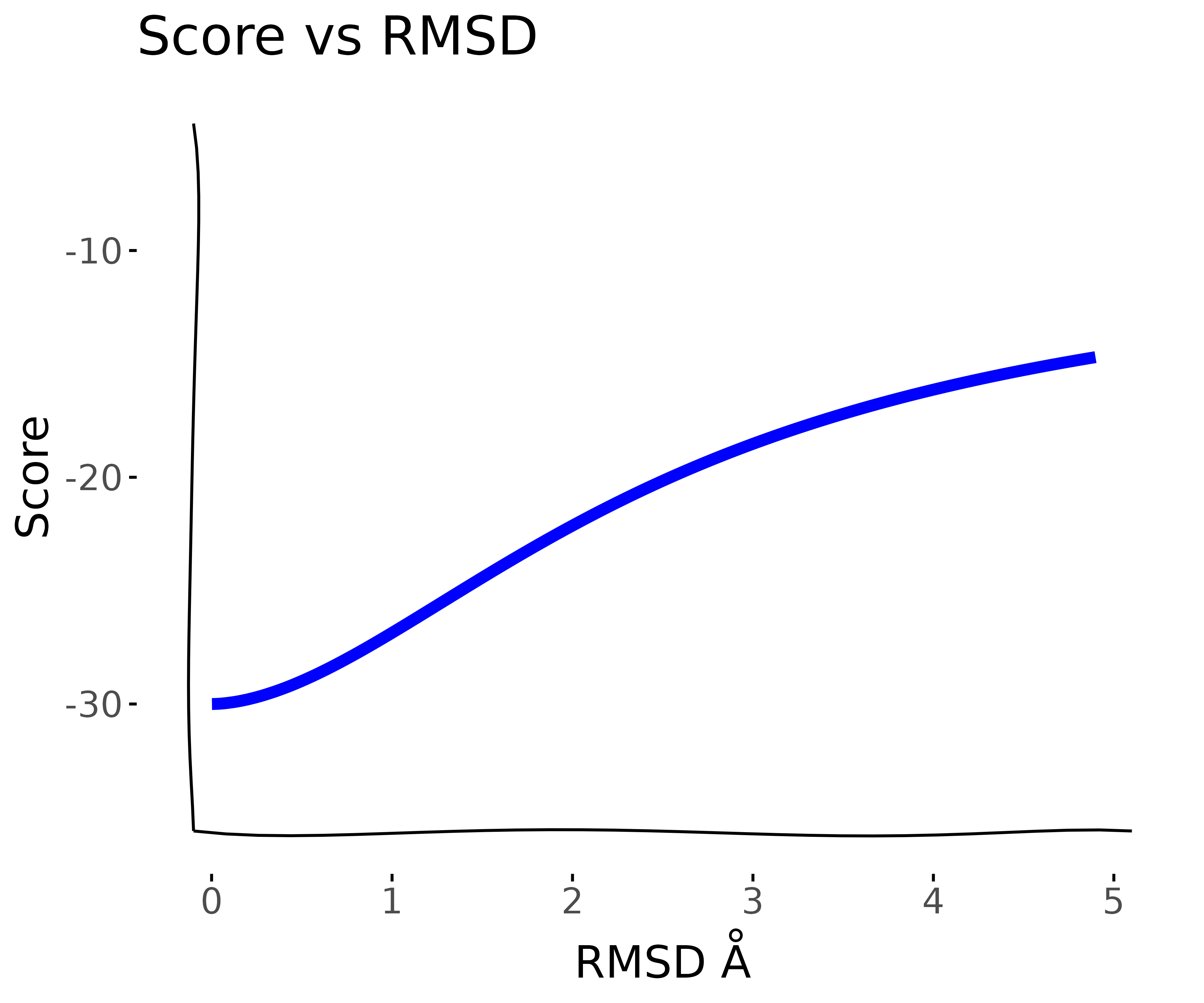
For a principled molecular dynamics or monte carlo simulation that maintains detailed balance, it is in theory possible to use thermodynamic integration to quantify the energy gap between the two states. However, this is often not computationally feasible for proteins of moderate size or in a protein design or screening context where many different molecules need to be evaluated given a limited computational budget. So, Instead, we will assume that the at least locally around the folded state, the degrees of freedom increase exponentially so that the log of the RMSD defines a linear reaction coordinate.
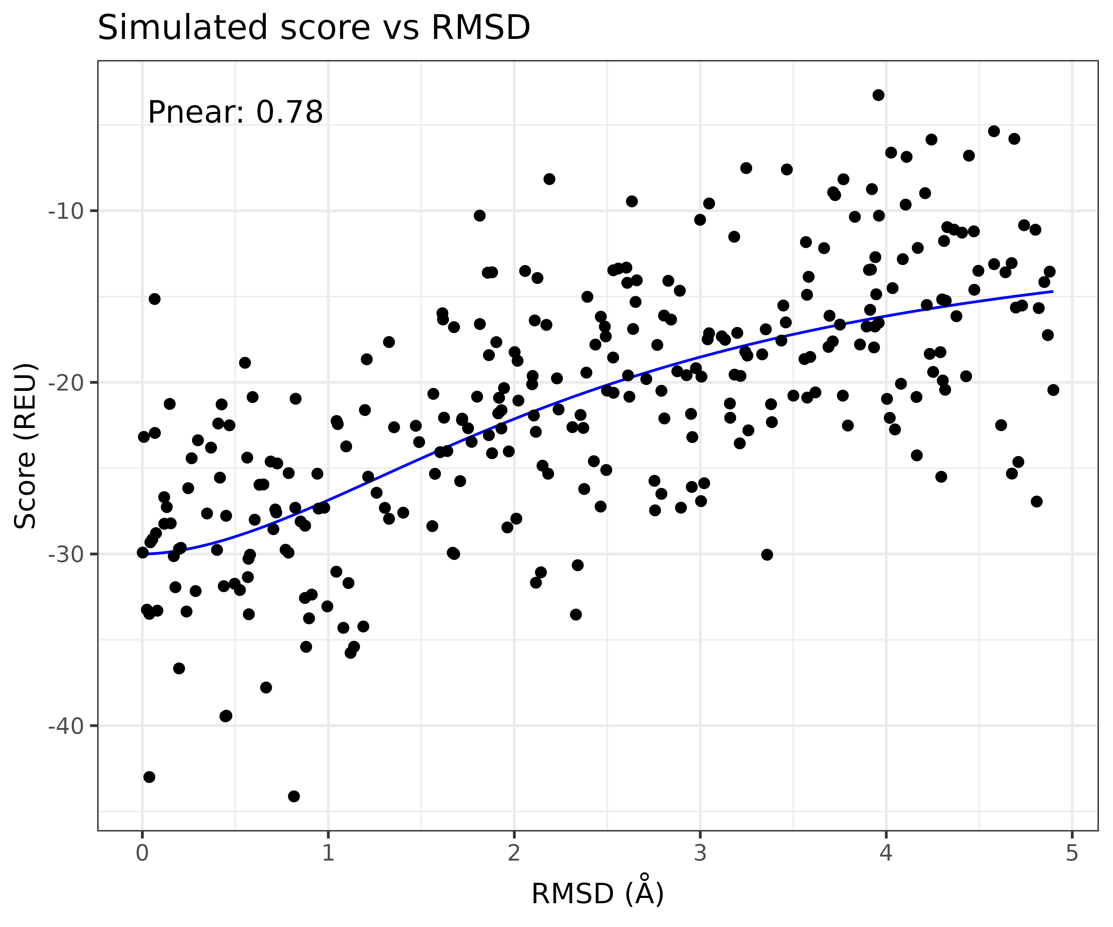
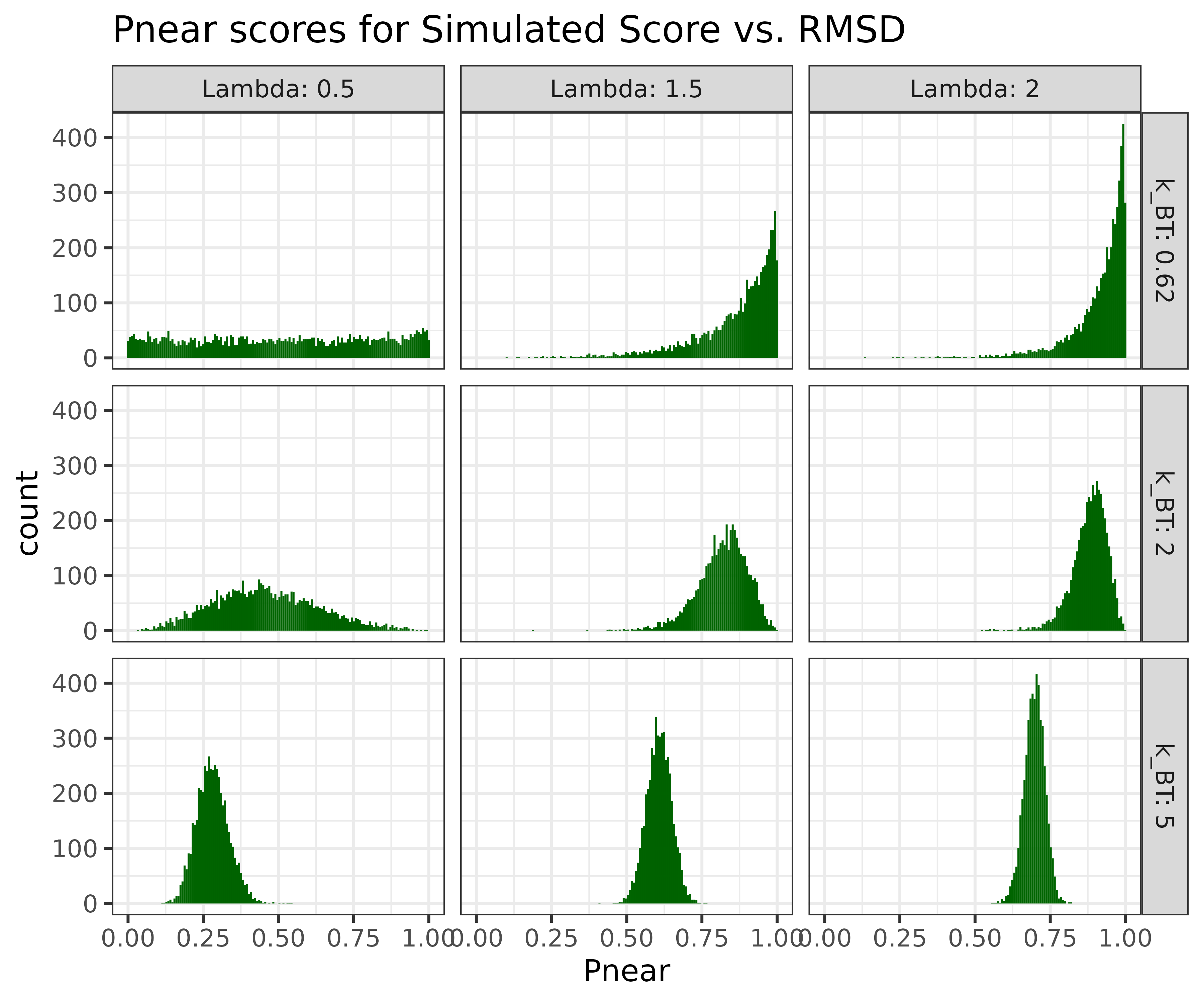
If we simulate, trajectory points from the sigmoid on the log(RMSD) scale, with a Normally distributed error we can generate synthetic score-vs-rmsd plots
A nice thing about having the parametric model to generate score-vs-rmsd plots, is that it allows us to measure measure the sensitivity of the Pnear to differently shaped score-vs-rmsd plots. For example we can scann both the radius of
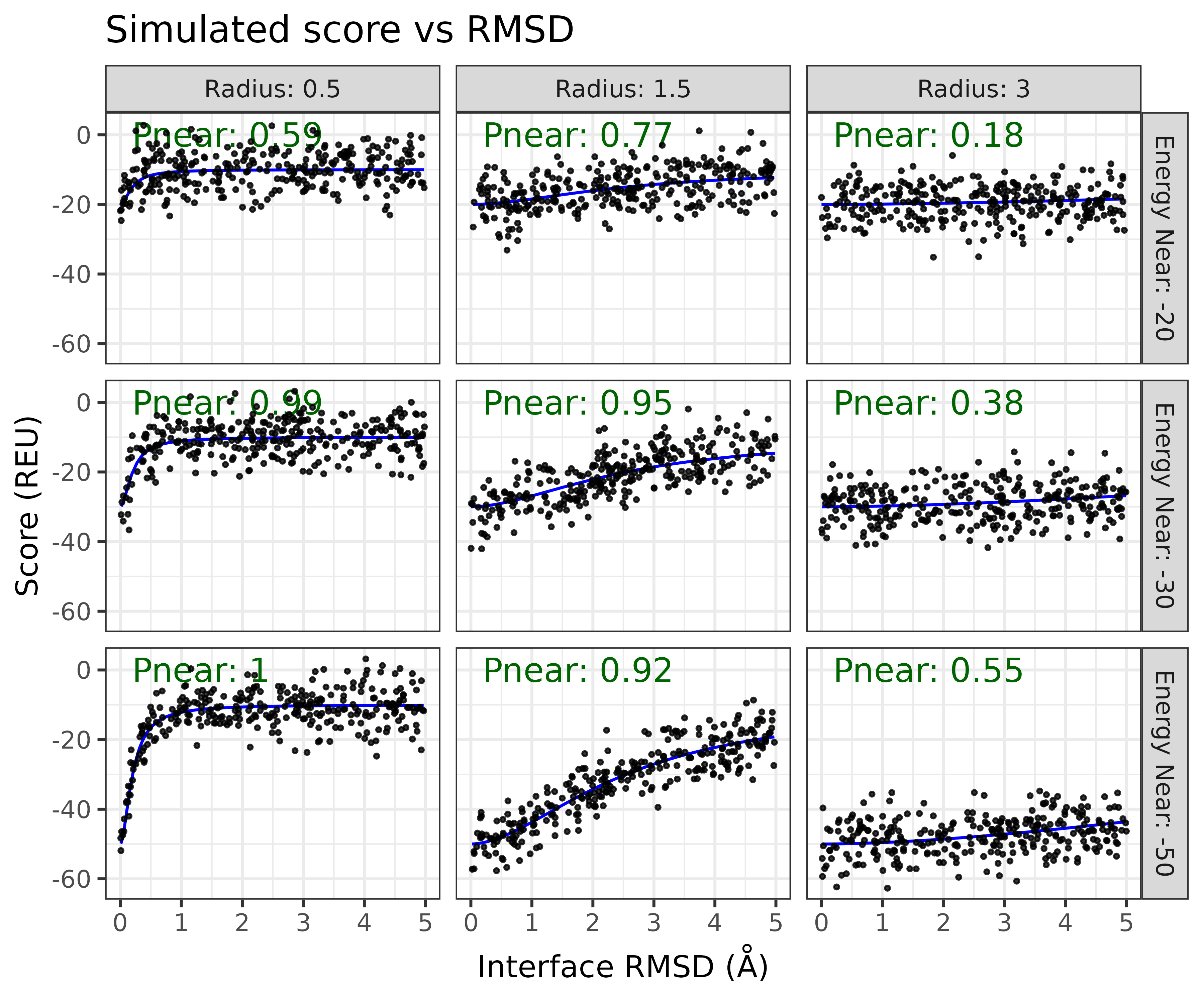
Another question we can use this model to investigate is how reproducible is the Pnear score?
Antibody SnugDock Case study
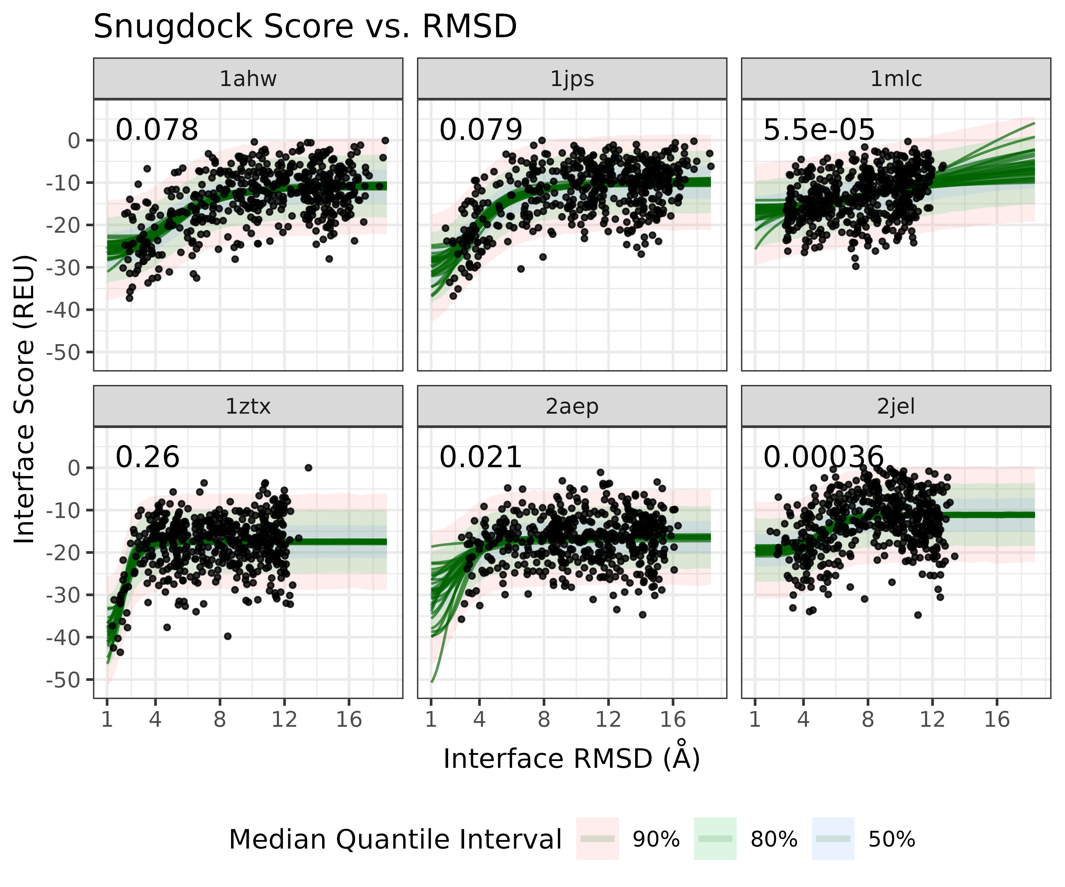
As a case study, we can look at the real score-vs-rmsd plots from the Antibody SnugDock scientific benchmark. It is evaluates the SnugDock protocol over 6 Antibody protein targets
We can use the fit the sigmoid model to the log(RMSD) using the BayesPharma package, which relies on BRMS and Stan
Check the model parameter fit and estimated parameters:
##  Family: gaussian
##   Links: mu = identity; sigma = identity
## Formula: response ~ sigmoid(ec50, hill, top, bottom, log_dose)
##          ec50 ~ 0 + target
##          hill ~ 0 + target
##          top ~ 0 + target
##          bottom ~ 0 + target
##    Data: data (Number of observations: 3003)
##   Draws: 4 chains, each with iter = 8000; warmup = 4000; thin = 1;
##          total post-warmup draws = 16000
##
## Population-Level Effects:
##                   Estimate Est.Error l-95% CI u-95% CI Rhat Bulk_ESS Tail_ESS
## ec50_target1ahw       1.70      0.11     1.45     1.87 1.00     8373     5054
## ec50_target1jps       1.37      0.13     1.09     1.59 1.00     8239     6806
## ec50_target1mlc       2.38      0.52     0.98     3.18 1.00     6420     4526
## ec50_target1ztx       0.75      0.08     0.59     0.89 1.00     9516     8256
## ec50_target2aep       1.11      0.29     0.59     1.50 1.00     7239     4493
## ec50_target2jel       1.65      0.06     1.53     1.76 1.00    10749     9119
## hill_target1ahw       1.69      0.44     0.90     2.62 1.00     5838     3539
## hill_target1jps       1.50      0.36     0.90     2.31 1.00     6985     6995
## hill_target1mlc       1.03      0.56     0.25     2.32 1.00     6094     6693
## hill_target1ztx       2.71      0.55     1.76     3.89 1.00    11766    10461
## hill_target2aep       2.00      0.66     0.74     3.39 1.00     6425     2509
## hill_target2jel       3.21      0.59     2.14     4.42 1.00    13407     9368
## top_target1ahw      -10.56      0.70   -11.57    -8.89 1.00     8065     4588
## top_target1jps       -9.71      0.57   -10.61    -8.35 1.00    10267     7705
## top_target1mlc       -1.32      5.91    -9.85    12.54 1.00    12538     9960
## top_target1ztx      -17.44      0.28   -17.98   -16.89 1.00    18000    11670
## top_target2aep      -16.31      0.76   -16.95   -15.48 1.00     6898     3192
## top_target2jel      -11.09      0.33   -11.74   -10.43 1.00    18945     9720
## bottom_target1ahw   -25.97      2.07   -31.09   -23.06 1.00     6374     3841
## bottom_target1jps   -30.46      3.70   -39.38   -24.89 1.00     7455     6840
## bottom_target1mlc   -18.55      4.45   -31.88   -14.74 1.00     5496     4294
## bottom_target1ztx   -38.92      3.52   -46.77   -33.08 1.00     9823     8023
## bottom_target2aep   -30.25      5.90   -43.62   -21.27 1.00    12150    10354
## bottom_target2jel   -19.45      0.98   -21.57   -17.72 1.00    11433     8658
##
## Family Specific Parameters:
##       Estimate Est.Error l-95% CI u-95% CI Rhat Bulk_ESS Tail_ESS
## sigma     5.74      0.07     5.60     5.89 1.00    20851    11865
##
## Draws were sampled using sampling(NUTS). For each parameter, Bulk_ESS
## and Tail_ESS are effective sample size measures, and Rhat is the potential
## scale reduction factor on split chains (at convergence, Rhat = 1).
Excitingly, using leave-one-out cross-validation, the sigmoid model fits the data very well
##
## Computed from 16000 by 3003 log-likelihood matrix
##
##          Estimate   SE
## elpd_loo  -9521.2 39.0
## p_loo        21.4  1.1
## looic     19042.5 78.0
## ------
## Monte Carlo SE of elpd_loo is 0.0.
##
## All Pareto k estimates are good (k < 0.5).
## See help('pareto-k-diagnostic') for details.
Visualize the fit as draws from the expected mean and median quantile intvervals on the log(RMSD) scale:
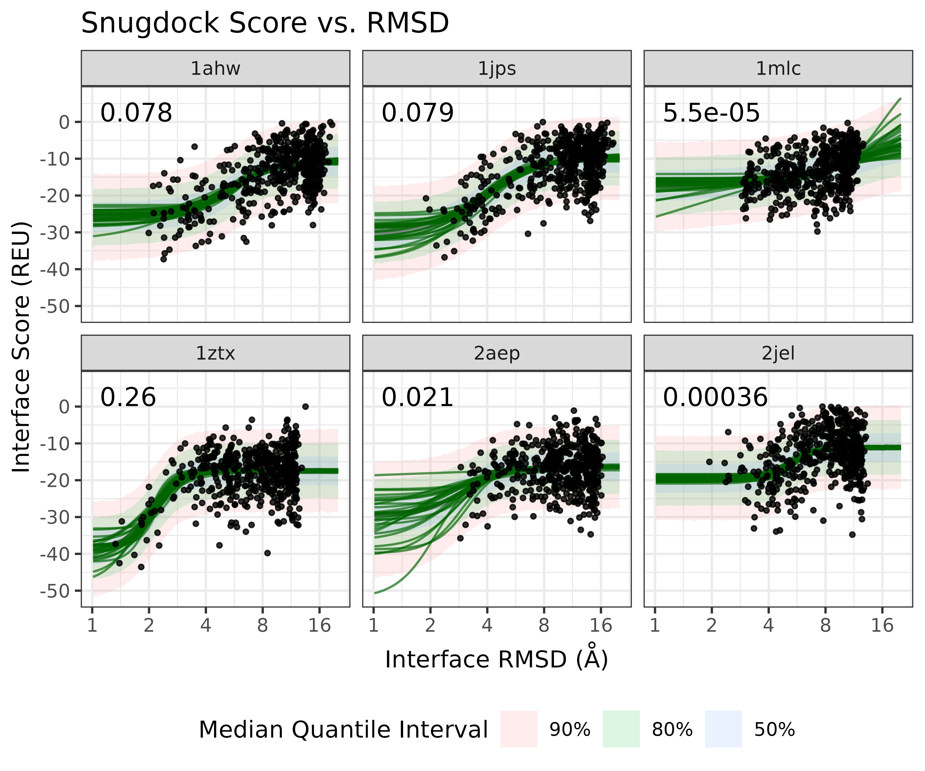 And on the original RMSD scale: