Apply: Sigmoid Model -- KOR Antagonists
Analysis of Four Kappa Opioid Receptor Antagonists
apply_sigmoid_model_KOR_antagonists.RmdHill Equation
In this case study we are going to reanalyze the dose response of 4
Kappa Opioid receptor (KOR) antagonists using the
BayesPharma package from from a study done by Margolis et
al. (-@Margolis2020-bm). Whole cell
electrophysiology in acute rat midbrain slices was used to evaluate
pharmacological properties of four novel KOR antagonists: BTRX-335140,
BTRX-395750, PF-04455242, and JNJ-67953964
Originally paper, the dose-response data analysis was done by using
the drc package in R which implements the minimization of
negative log likelihood function and reduces to least square estimation
for a continuous response. The data was normalized to % baseline then
fit to a 4-parameter log-logistic dose response model, setting the top
(max response) to 100% and estimating the IC50, its variance, and the
bottom (min response).
Fitting the sigmoid model
Using the BayesPharma package, we can re-fit the sigmoid model with a negative slope, and fixing the top parameter to 100 as the response is normalized to a no-drug baseline.
For the prior, we are going to use a normal distribution because the response values are continuous. First, We will run the analysis with top (max response) parameter prior set to a constant value of 100 because top is normalized to 100 and the default broad prior for ic50, hill and bottom. Broad priors represent unbiased uncertainty and provide an opportunity for extreme responses.
The level of informativeness of the prior will affect how much influence the prior has on the model. Here is more information on prior choice recommendations.
kor_prior <- BayesPharma::sigmoid_antagonist_prior(top = 100)
kor_prior
##            prior class coef group resp dpar  nlpar   lb   ub source
##  normal(-6, 2.5)     b                        ic50 <NA> <NA>   user
##    normal(-1, 1)     b                        hill <NA> 0.01   user
##    constant(100)     b                         top <NA> <NA>   user
##   normal(0, 0.5)     b                      bottom <NA> <NA>   user
Prior predictive checks
Following the Bayesian workflow, before fitting the model it is good
to check the prior predictive distributions to see if they are
compatible with the domain expertise. So, before running the model, we
will verify that the prior distributions cover a plausible range of
values for each parameter. To do this, we want to sample only from the
prior distributions by adding sample_prior = “only” as an
argument to the sigmoid_antagonist_model function. We will
use the default response distribution of the model (family =
gaussian()).
kor_sample_prior <- BayesPharma::sigmoid_antagonist_model(
  data = kor_antag |> dplyr::select(substance_id, log_dose, response),
  prior = kor_prior,
  sample_prior = "only")
And then plot of the prior predictive distributions:
kor_sample_prior |>
  BayesPharma::density_distributions_plot()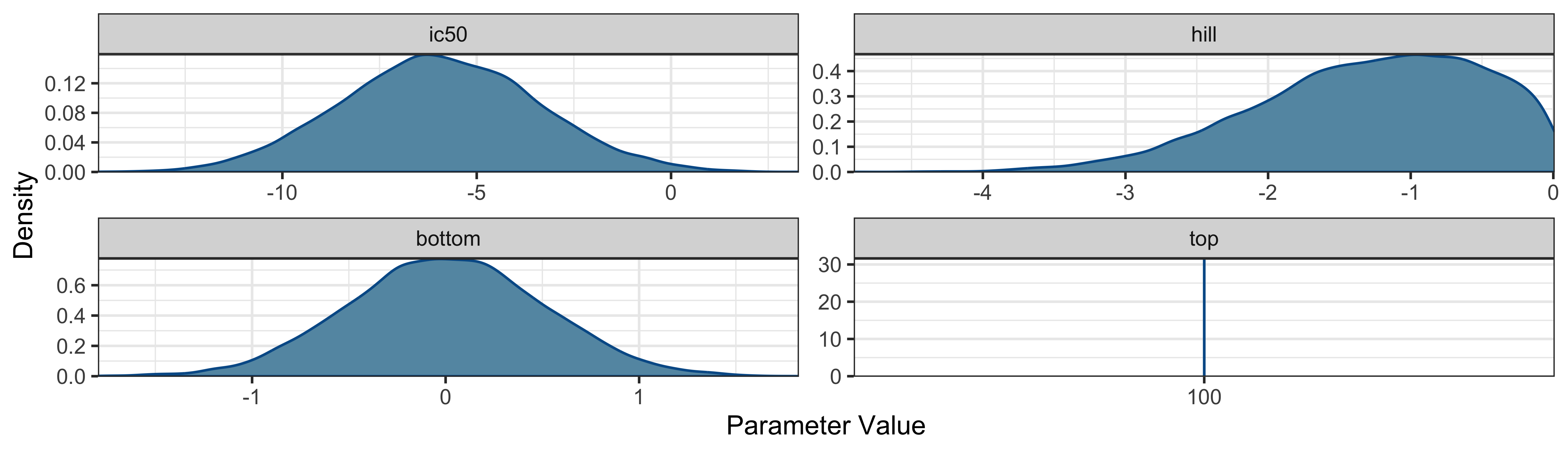
To sample from the model we will the Stan NUTs Hamiltonian Monte Carlo, and initialize the parameters to the prior means to help with model convergence, using the default values of ec50 = -9, hill = -1, top = 100, bottom = 0.
kor_model <- BayesPharma::sigmoid_antagonist_model(
  data = kor_antag |> dplyr::select(substance_id, log_dose, response),
  formula = BayesPharma::sigmoid_antagonist_formula(
    predictors = 0 + substance_id),
  prior = kor_prior)
Analyzing model fit
The BRMS generated model summary shows the formula that the expected
response is sigmoid function of the log_dose with four parameters, and a
shared Gaussian distribution. Each parameter is dependent on the
substance_id. Since want to fit a separate model for each substance we
include a 0 + to indicate that there is no common
intercept. The consists of 73 data points and the posterior sampling was
done in 4 chains each with 8000 steps with 4000 steps of warm-up. The
population effects for each parameter summarize marginal posterior
distributions, as well as the effective sample size in the bulk and
tail. This gives an indication of the sampling quality, with an ESS of
> 500 samples being good for this type of model.
##  Family: gaussian
##   Links: mu = identity; sigma = identity
## Formula: response ~ sigmoid(ic50, hill, top, bottom, log_dose)
##          ic50 ~ 0 + substance_id
##          hill ~ 0 + substance_id
##          top ~ 0 + substance_id
##          bottom ~ 0 + substance_id
##    Data: data (Number of observations: 73)
##   Draws: 4 chains, each with iter = 8000; warmup = 4000; thin = 1;
##          total post-warmup draws = 16000
##
## Population-Level Effects:
##                                Estimate Est.Error l-95% CI u-95% CI Rhat Bulk_ESS Tail_ESS
## ic50_substance_idBTRX_335140      -8.84      0.20    -9.20    -8.40 1.00    14883     8873
## ic50_substance_idBTRX_395750      -8.24      0.41    -8.92    -7.39 1.00    12333     5863
## ic50_substance_idJNJ              -9.15      0.32    -9.78    -8.50 1.00    17511    10242
## ic50_substance_idPF               -6.15      1.05    -7.64    -3.41 1.00     8649     6213
## hill_substance_idBTRX_335140      -1.47      0.60    -2.89    -0.59 1.00    15340    10545
## hill_substance_idBTRX_395750      -0.89      0.51    -2.24    -0.26 1.00    12763     6273
## hill_substance_idJNJ              -1.01      0.51    -2.38    -0.41 1.00    15285    11508
## hill_substance_idPF               -0.31      0.24    -0.88    -0.03 1.00     7904     4559
## bottom_substance_idBTRX_335140    -0.00      0.50    -0.99     0.97 1.00    19984    11491
## bottom_substance_idBTRX_395750     0.01      0.50    -0.97     1.00 1.00    19123    11247
## bottom_substance_idJNJ            -0.01      0.50    -0.98     0.98 1.00    18940    11984
## bottom_substance_idPF              0.00      0.50    -0.98     0.98 1.00    21351    12102
## top_substance_idBTRX_335140      100.00      0.00   100.00   100.00   NA       NA       NA
## top_substance_idBTRX_395750      100.00      0.00   100.00   100.00   NA       NA       NA
## top_substance_idJNJ              100.00      0.00   100.00   100.00   NA       NA       NA
## top_substance_idPF               100.00      0.00   100.00   100.00   NA       NA       NA
##
## Family Specific Parameters:
##       Estimate Est.Error l-95% CI u-95% CI Rhat Bulk_ESS Tail_ESS
## sigma    32.17      2.84    27.19    38.32 1.00    14690    10539
##
## Draws were sampled using sampling(NUTS). For each parameter, Bulk_ESS
## and Tail_ESS are effective sample size measures, and Rhat is the potential
## scale reduction factor on split chains (at convergence, Rhat = 1).
Traceplot
The model ran without warning messages meaning there were no parameter value problems or mcmc conflicts. The bulk and tail ESS indicate high resolution and stability. The R-hat for each parameter equals 1.00 and the traceplot shows the chains mixed well indicating the chains converged.
kor_model |>
  bayesplot::mcmc_trace()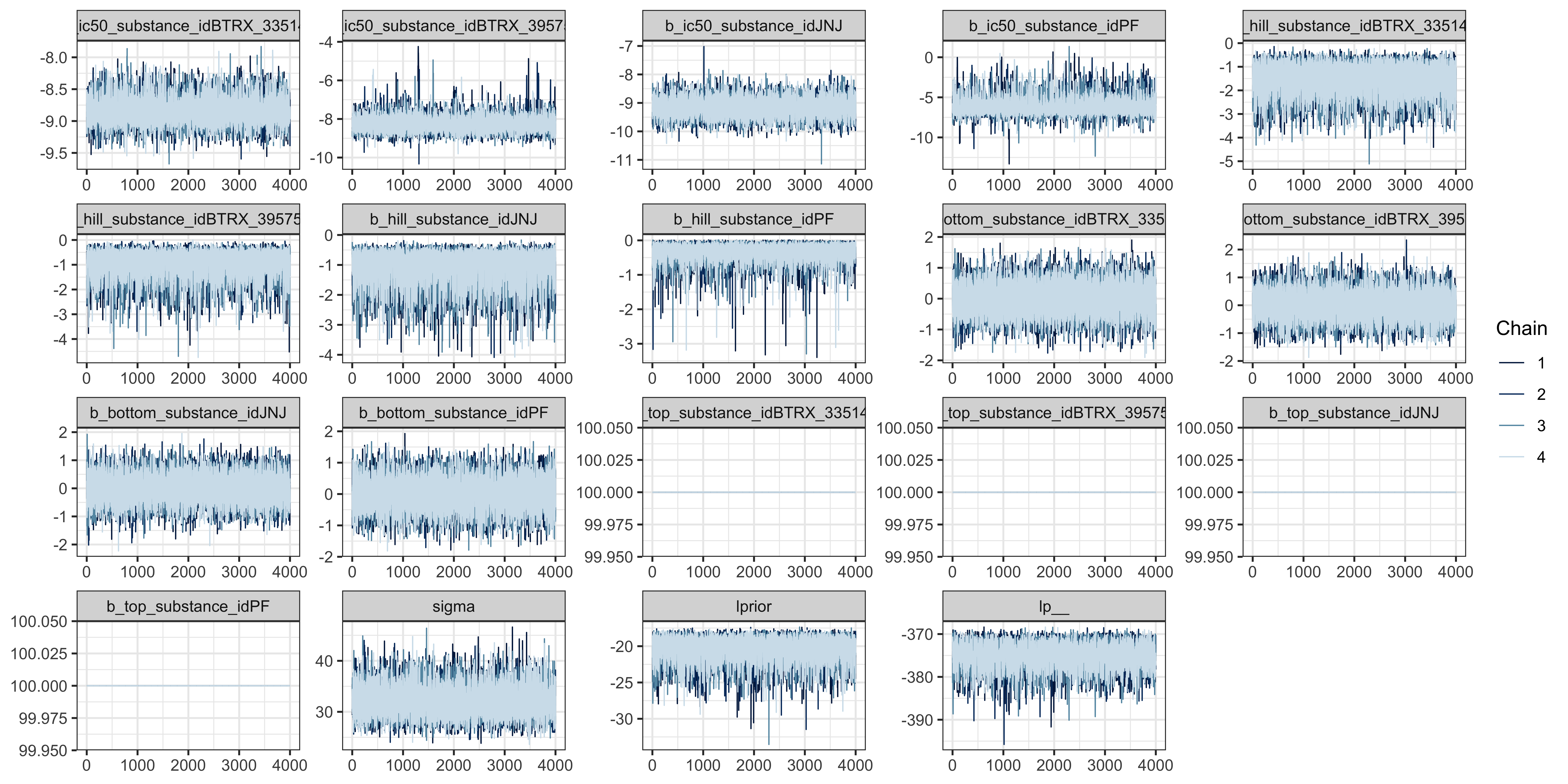
Compare prior and posterior marginal distributions
Displayed below is a plot for the prior and posterior distributions of the parameters (prior is pink and posterior is teal). this can be useful for comparing the density distribution of the prior and posterior. produced by the model:
BayesPharma::prior_posterior_densities_plot(
  model = kor_model,
  predictors_col_name = "substance_id",
  half_max_label = "ic50",
  title_label="")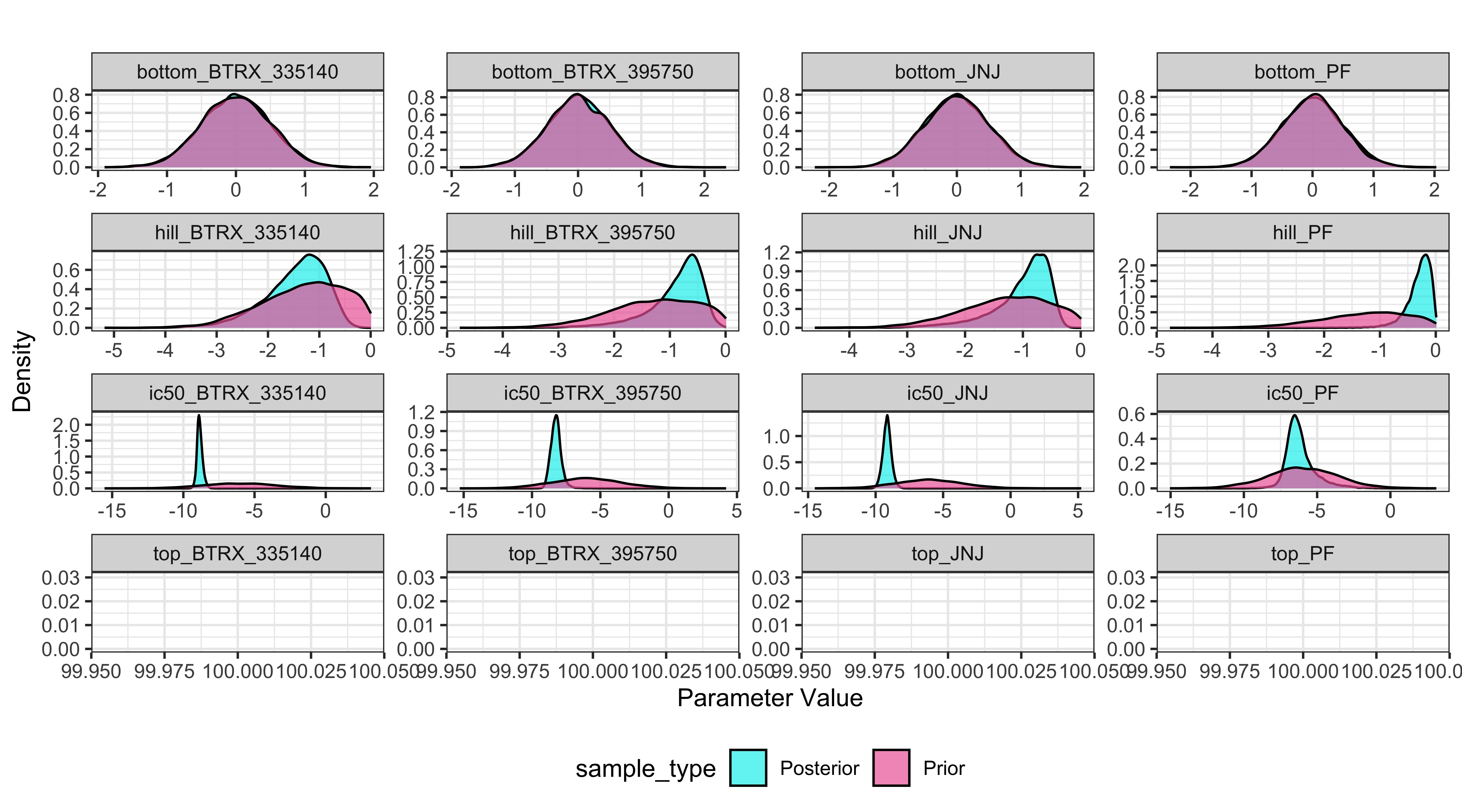
Displayed below is a plot of the posterior distributions for each parameter with the confidence intervals and mean. This is a useful visual of the model results and to highlight the mode and high density intervals:
BayesPharma::posterior_densities_plot(
  kor_model,
  predictors_col_name = "substance_id",
  half_max_label = "ic50",
  title_label = "")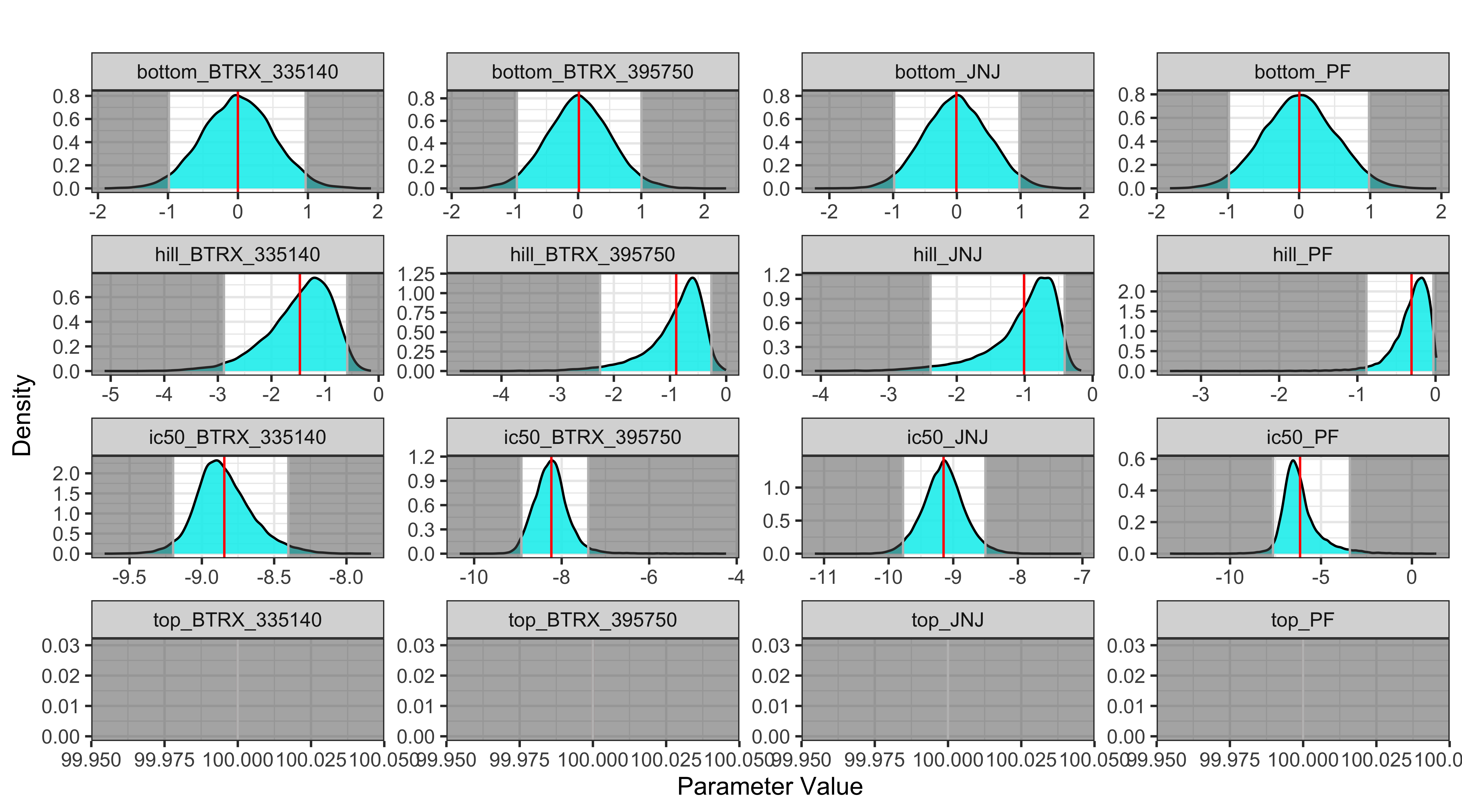
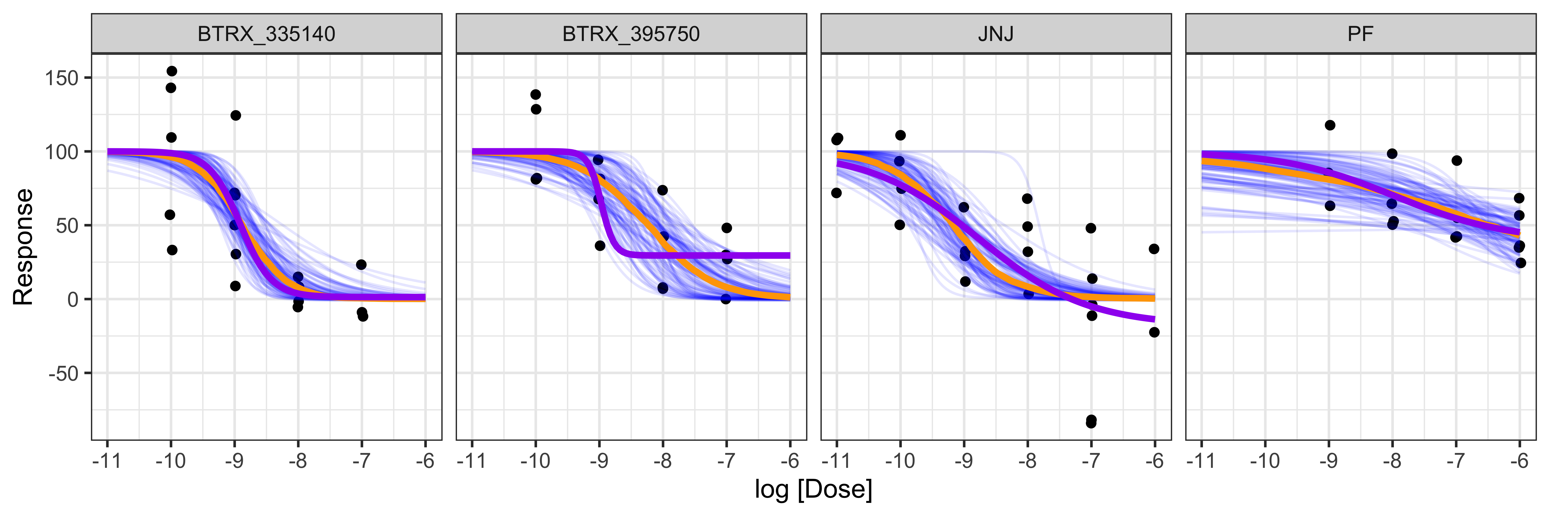
Displayed below is a plot of a sample of 100 sigmoid dose-response curves from the posterior distribution (purple) and the median quantile intervals:
BayesPharma::posterior_draws_plot(
  model = kor_model,
  title = "")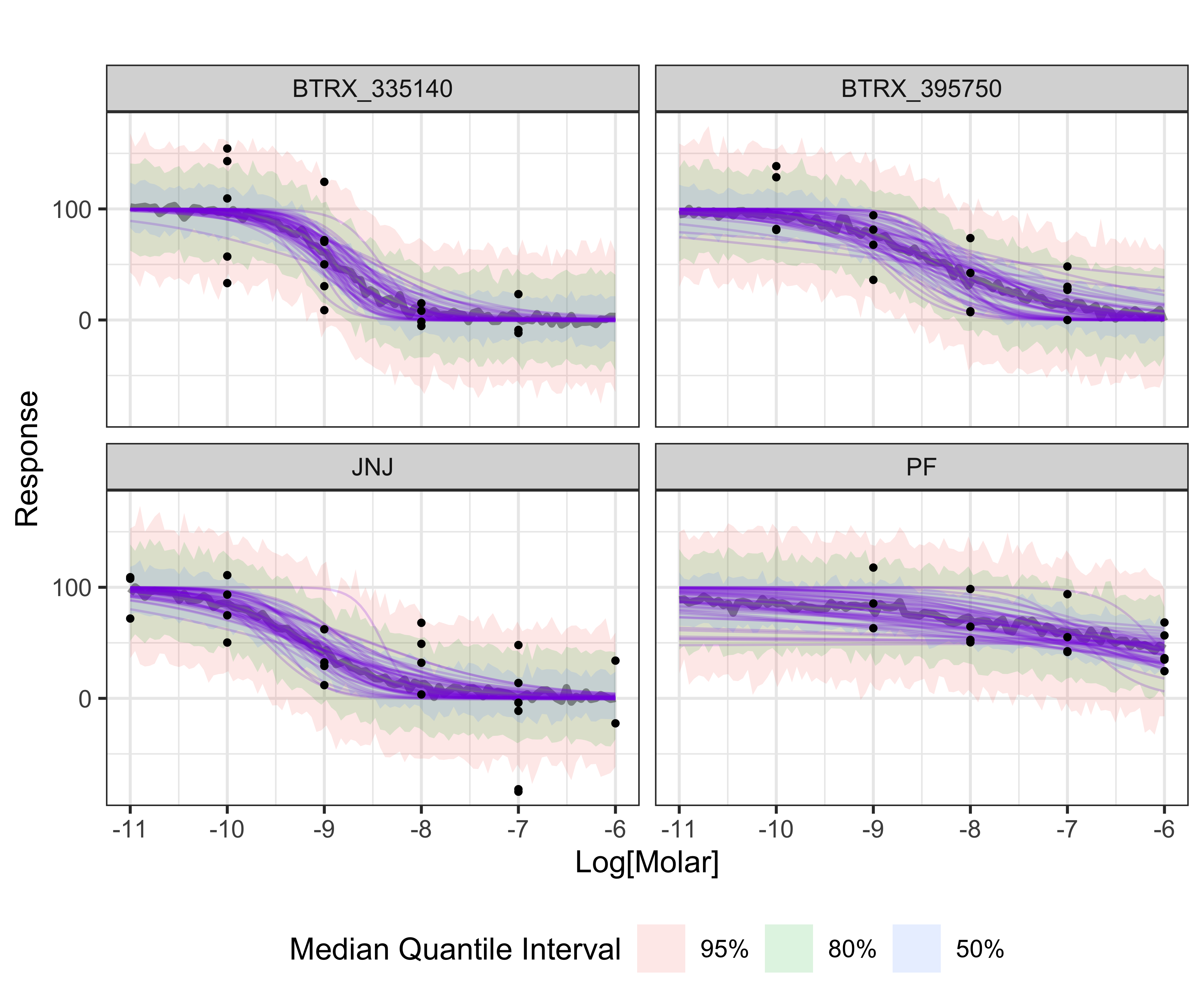
Comparing alternative models
To test the sensitivity of the analysis to the prior, we can re-fit the model with more informative prior:
##            prior class coef group resp dpar  nlpar   lb   ub source
##  normal(-6, 2.5)     b                        ic50 <NA> <NA>   user
##  normal(-1, 0.5)     b                        hill <NA> 0.01   user
##    constant(100)     b                         top <NA> <NA>   user
##   normal(10, 15)     b                      bottom <NA> <NA>   user
Re-fitting the model
Comparing the Two Models Using LOO-Comparison:
One way to evaluate the quality of a model is for each data-point, re-fit the model with remaining points, and evaluate the log probability of the point in the posterior distribution. Taking the expectation across all points give the Expected Log Pointwise predictive Density (ELPD). Since this is computationally challenging to re-fit the model for each point, if the model fits the data reasonably well, then the ELPD can be approximated using the Pareto smoothed importance sampling (PSIS). Using the LOO, the package, Pareto k value for each data point is computed, where k less than 0.5 is good, between 0.5 and 0.7 is ok, and higher than 0.7 indicates the data point is not fit by the model well. Evaluating the model for the KOR antagonists, shows that the model fits the data well.
## No problematic observations found. Returning the original 'loo' object.
## NULL
Since ELPD is a global measure of model fit, it can be used to
compare models. Using loo_compare from the LOO package,
returns the elpd_diff and se_diff for each
model relative the model with the lowest ELPD. The
kor_model2, the model with more informative prior, is the
preferred model, but not significantly.
## No problematic observations found. Returning the original 'loo' object.
##            elpd_diff se_diff
## kor_model   0.0       0.0
## kor_model2 -0.2       0.8
##Analysis Using the drc Package
Here we will analyze the KOR antagonist data using the drc package and compare it to the results from the BayesPharma analysis.
We will fix the top to 100 and fit the ic50, hill, and bottom.
drc_models <- kor_antag |>
  dplyr::group_by(substance_id) |>
  dplyr::group_nest() |>
  dplyr::mutate(
    model = data |>
      purrr::map(~drc::drm(
        response ~ log_dose,
        data = .x,
        fct = drc::L.4(fixed = c(NA, NA, 100, NA),
        names = c("hill", "bottom", "top", "ic50")))))

drc_models |>
  dplyr::mutate(summary = purrr::map(model, broom::tidy, conf.int = TRUE)) |>
  tidyr::unnest(summary) |>
  dplyr::arrange(term, substance_id) |>
  dplyr::select(-data, -model, -curve)
## # A tibble: 12 × 8
##    substance_id term   estimate std.error statistic  p.value  conf.low conf.high
##    <chr>        <chr>     <dbl>     <dbl>     <dbl>    <dbl>     <dbl>     <dbl>
##  1 BTRX_335140  bottom     1.31    19.4      0.0675 9.47e- 1  -40.0        42.6
##  2 BTRX_395750  bottom    29.5      9.40     3.14   7.85e- 3    9.20       49.8
##  3 JNJ          bottom   -18.1     26.7     -0.681  5.04e- 1  -73.7        37.4
##  4 PF           bottom    39.4     30.8      1.28   2.22e- 1  -27.0       106.
##  5 BTRX_335140  hill       4.06     9.20     0.441  6.65e- 1  -15.5        23.7
##  6 BTRX_395750  hill       9.82   164.       0.0600 9.53e- 1 -344.        364.
##  7 JNJ          hill       1.17     0.580    2.02   5.69e- 2   -0.0378      2.38
##  8 PF           hill       1.13     1.33     0.855  4.08e- 1   -1.73        4.00
##  9 BTRX_335140  ic50      -8.91     0.308  -28.9    1.42e-14   -9.57       -8.26
## 10 BTRX_395750  ic50      -8.97     0.505  -17.8    1.70e-10  -10.1        -7.88
## 11 JNJ          ic50      -8.77     0.670  -13.1    2.89e-11  -10.2        -7.37
## 12 PF           ic50      -7.96     1.27    -6.29   2.78e- 5  -10.7        -5.23
Displayed below is the comparison of results from drc
and BayesPharma for each parameter of the dose-response
curve. Here we see that the Bayesian method provides a distribution
curve as evidence and has smaller confidence intervals than most of the
standard errors provided by the drc method.
## Warning: Using `size` aesthetic for lines was deprecated in ggplot2 3.4.0.
## ℹ Please use `linewidth` instead.