Derive: tQ Model -- Enzyme Kinetics

## Error in library(tidyverse): there is no package called 'tidyverse'

Enzyme Kinetic Modeling

Enzymes are proteins that catalyze chemical reactions. Not only do they facilitate producing virtual all biological matter, but they are crucial for regulating biological processes. In the early 20th century Michaelis and Menten described a foundational kinematic model for enzymes, where the substrate and enzyme reversibly bind, the substrate is converted to the product and then released.

              kf
             --->     kcat
      E + S  <---  C --->  E + P
              kb

where the free enzyme (E) reversibly binds to the stubstrate (S) to form a complex (C) with forward and backward rate constants of kf and kb, which is irreversibly catalyzed into the product (P), with rate constant of kcat, releasing the enzyme to catalyze additional substrate. The total enzyme concentration is defined to be the ET := E + C. The total substrate and product concentration is defined to be ST := S + C + P. The Michaelis constant is the defined to be the kM := (kb + kcat) / kf. The kcat rate constant determines the maximum turn over at saturating substrate concentrations, Vmax := kcat * ET. The rate constants kcat and kM can be estimated by monitoring the product accumulation over time (enzyme progress curves), by varying the enzyme and substrate concentrations.

By assuming that the enzyme concentration is very low (ET << ST), they derived their celebrated Michaelis-Menten kinetics. Since their work, a number of groups have developed models for enzyme kinetics that make less stringent assumptions. Recently (Choi, et al., 2017), described a Bayesian model for the total QSSA model. To make their model more accessible, we have re-implemented it in the Stan/BRMS framework and made it available through the BayesPharma package.

Outline for Vignette

Next we will formally define the problem and formulate the model as the solution to an ordinary differential equation. To illustrate, we will consider a a toy system where we assuming the kcat and kM are known and simulate a sequence of measurements using deSolve. We will then implement the ODE in Stan/BRMS using stanvars and show how the parameters of the toy system can be estimated. Since it is common to vary the enzyme and substrate concentrations in order to better estimate the kinematic parameters, we will show how we can improve the Stan/BRMS model to allow multiple observations, each with an arbitrary number of measurements. Then finally, we will consider a real enzyme kinetics data set and use the Stan/BRMS model to estimate the kinematic parameters. We will compare estimated parameters with those fit using standard approaches.

Problem Statement

Implement the total QSSA model in stan/BRMS, a refinement of the classical Michaelis-Menten enzyme kinetics ordinary differential equation described in (Choi, et al., 2017, DOI: 10.1038/s41598-017-17072-z). From their equation 2:

Observed data:
  M     = number of measurements # The product concentration Pt is measured
  t[M]  = time                   # at M time points t
  Pt[M] = product                # 
  ST    = substrate total conc.  # Substrate and enzyme concentrations are
  ET    = enzyme total conc.     # assumed to be given for each observation

Model parameters:
  kcat    # catalytic constant
  kM      # Michaelis constant

ODE formulation:
  dPdt = kcat * (                # Change in product concentration at time t
    ET + kM + ST - Pt +          
    -sqrt((ET + kM + ST - Pt)^2 - 2* ET * (ST - Pt))) / 2
  initial condition:
    P := 0                       # There is zero product at time 0

In (Choi, et al. 2017) they prove, that the tQ model is valid when

 K/(2*ST) * (ET+kM+ST) / sqrt((ET+kM+ST+P)^2 - 4*ET(ST-P)) << 1,

where K = kb/kf is the dissociation constant.

Simulate one observation

Using the deSolve package we can simulate data following the total QSSA model. Measurements are made with random Gaussian noise with mean 0 and variance of 0.5.

tQ_model_generate <- function(time, kcat, kM, ET, ST){
  ode_tQ <- function(time, Pt, theta){
    list(c(theta[1] * (
      ET + theta[2] + ST - Pt +
      -sqrt((ET + theta[2] + ST - Pt)^2 - 4 * ET * (ST - Pt))) / 2))
  }
  deSolve::ode(y = 0, times = time, func = ode_tQ, parms = c(kcat, kM))
}

data_single <- tQ_model_generate(
  time = seq(0.00, 3, by=.05),
  kcat = 3,
  kM = 5,
  ET = 10,
  ST = 10) |>
  as.data.frame() |>
  dplyr::rename(P_true = 2) |>
  dplyr::mutate(
    P = rnorm(dplyr::n(), P_true, 0.5), # add some observational noise
    ST = 10, ET = 10)
head(data_single)

##   time    P_true         P ST ET
## 1 0.00 0.0000000 0.1223538 10 10
## 2 0.05 0.7311578 0.6060729 10 10
## 3 0.10 1.4243598 2.0420722 10 10
## 4 0.15 2.0794197 2.3973591 10 10
## 5 0.20 2.6964485 2.1516463 10 10
## 6 0.25 3.2758537 3.3034788 10 10

To visualize, the true enzyme progress curve is shown in blue, and the enzyme progress curve fit to the noisy measurements with a smooth loess spline is shown in orange. While the smooth fits well, we cannot estimate the parameters for the curve from it.

## Warning: Using `size` aesthetic for lines was deprecated in ggplot2 3.4.0.
## ℹ Please use `linewidth` instead.
## This warning is displayed once every 8 hours.
## Call `lifecycle::last_lifecycle_warnings()` to see where this warning was generated.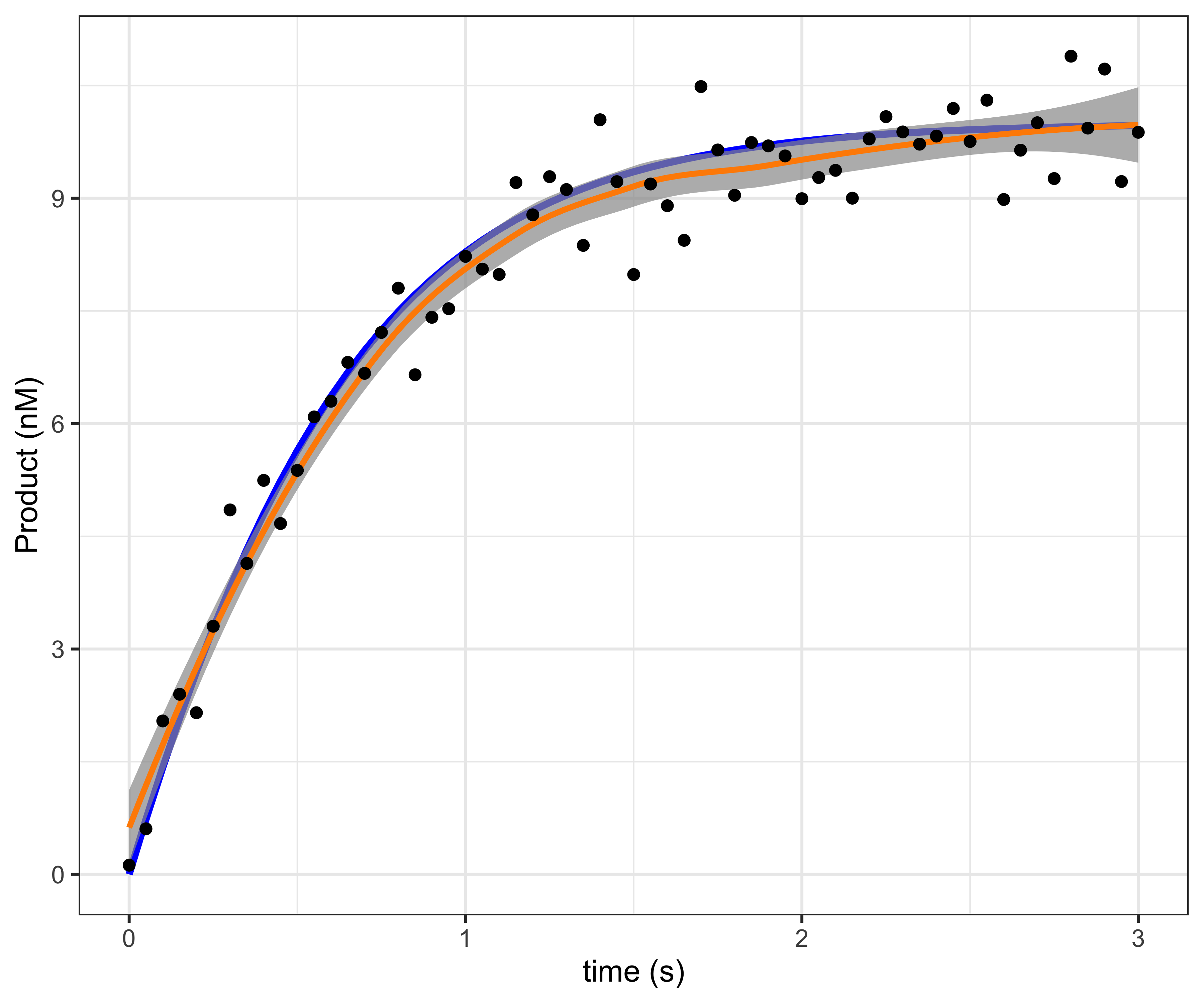

plot of chunk data-single-plot

Fitting a single ODE observation in BRMS

To implement in BRMS, we can use the stanvars to define custom functions. The key idea is call the ODE solver, in this case the backward differentiation formula (bdf) used to solve stiff ODEs, passing a function ode_tQ that returns dP/dt, the change in product at time t. The ode_tQ function depends on the product at time t as the state vector, the kinematic parameters to be estimated kcat and kM and the user-provided data of the enzyme and substrate concentrations ET and ST. To call ode_dbf we pass in the initial product concentration and time (both equal to zero), measured time-points, parameters and user defied data. Finally we, extract the vector of sampled vector of product concentrations which we return.

stanvars_tQ_ode <- brms::stanvar(scode = paste("
vector tQ_ode(
   real time,
   vector state,
   vector params,
   data real ET,
   data real ST) {
   
   real Pt = state[1];   // product at time t
   real kcat = params[1];
   real kM = params[2];
   vector[1] dPdt;
   dPdt[1] = kcat * (
     ET + kM + ST - Pt
     -sqrt((ET + kM + ST - Pt)^2 - 4 * ET * (ST - Pt))) / 2;
   return(dPdt);
}
", sep = "\n"),
block = "functions")

stanvars_tQ_single <- brms::stanvar(scode = paste("
vector tQ_single(
  data vector time,
  vector vkcat,
  vector vkM,
  data vector vET,
  data vector vST) {
  
  vector[2] params = [ vkcat[1], vkM[1] ]';
  vector[1] initial_state = [ 0.0 ]';
  real initial_time = 0.0;
  int M = dims(time)[1];

  vector[1] P_ode[M] = ode_bdf(     // Function signature:
    tQ_ode,                         // function ode
    initial_state,                  // vector initial_state
    initial_time,                   // real initial_time
    to_array_1d(time),              // array[] real time
    params,                         // vector params
    vET[1],                         // ...
    vST[1]);                        // ...
  
  vector[M] P;                      // Need to return a vector not array
  for(i in 1:M) P[i] = P_ode[i,1];
  return(P);
}
", sep = "\n"),
block = "functions")

To use this function, we define kcat and kM as parameters and that we wish to sample P ~ tQ(...). Since all the data points define a single observation, we set loop = FALSE. We use gamma priors for kcat and kM with the shape parameter alpha=4 and the rate parameter beta=1. The prior mean is alpha/beta = 4/1 = 4 and the variance is alpha/beta^2 = 4/1 = 4. We also bound the parameters from below by 0. We initialize each chain at the prior mean and use cmdstanr version 2.29.2 as the backend, and use the default warmup of 1000

brms_params <- list(
  cores = 4,
  seed = 52L,
  backend = 'cmdstanr')

model_single <- do.call(what = brms::brm, args = c(list(
  formula = brms::brmsformula(
    P ~ tQ_single(time, kcat, kM, ET, ST),
    kcat + kM ~ 1,
    nl = TRUE,
    loop=FALSE),
  data = data_single |> dplyr::filter(time > 0),
  prior = c(
    brms::prior(prior = gamma(4, 1), lb = 0, nlpar = "kcat"),
    brms::prior(prior = gamma(4, 1), lb = 0, nlpar = "kM")),
  init = function() list(kcat = 4, kM = 4),
  stanvars = c(
    stanvars_tQ_ode,
    stanvars_tQ_single)),
  brms_params))

## Warning in '/var/folders/w2/kpys2s194q381xp3_knz9bgc0000gs/T/RtmpFnbbA1/model-141037b56c0ad.stan', line 34, column 2: Declaration
##     of arrays by placing brackets after a variable name is deprecated and
##     will be removed in Stan 2.33.0. Instead use the array keyword before the
##     type. This can be changed automatically using the auto-format flag to
##     stanc

## error: PCH file uses an older PCH format that is no longer supported

## Warning: CmdStan's precompiled header (PCH) files may need to be rebuilt.
## If your model failed to compile please run rebuild_cmdstan().
## If the issue persists please open a bug report.

## 1 error generated.
## make[1]: *** [/var/folders/w2/kpys2s194q381xp3_knz9bgc0000gs/T/RtmpFnbbA1/model-141037b56c0ad] Error 1

## Error: An error occured during compilation! See the message above for more information.

Fitting the model takes ~15 seconds, with Rhat = 1 and effective sample size for the bulk and tail greater than 1400 for both parameters. The estimates and 95% confidence intervals are good.

## Error in eval(expr, envir, enclos): object 'model_single' not found

To visualize the posterior distribution vs. the prior distribution, we first sample from the prior, using the same brms::brm call with sample_prior = "only" the argument.

model_single_prior <- do.call(what = brms::brm, args = c(list(
  formula = brms::brmsformula(
    P ~ tQ_single(time, kcat, kM, ET, ST),
    kcat + kM ~ 1,
    nl = TRUE,
    loop=FALSE),
  data = data_single |> dplyr::filter(time > 0),
  prior = c(
    brms::prior(prior = gamma(4, 1), lb = 0, nlpar = "kcat"),
    brms::prior(prior = gamma(4, 1), lb = 0, nlpar = "kM")),
  init = function() list(kcat = 4, kM = 4),
  stanvars = c(
    stanvars_tQ_ode,
    stanvars_tQ_single),
  sample_prior = "only"),
  brms_params))

## Warning in '/var/folders/w2/kpys2s194q381xp3_knz9bgc0000gs/T/RtmpFnbbA1/model-1410319141a6d.stan', line 34, column 2: Declaration
##     of arrays by placing brackets after a variable name is deprecated and
##     will be removed in Stan 2.33.0. Instead use the array keyword before the
##     type. This can be changed automatically using the auto-format flag to
##     stanc

## error: PCH file uses an older PCH format that is no longer supported

## Warning: CmdStan's precompiled header (PCH) files may need to be rebuilt.
## If your model failed to compile please run rebuild_cmdstan().
## If the issue persists please open a bug report.

## 1 error generated.

## make[1]: *** [/var/folders/w2/kpys2s194q381xp3_knz9bgc0000gs/T/RtmpFnbbA1/model-1410319141a6d] Error 1

## Error: An error occured during compilation! See the message above for more information.

And to plot, we use tidybayes to gather the draws and ggplot2 to map them to curves, with the prior as theorange curve, posterior as the blue curve, and the true parameter marked as a vertical line.

## Error in eval(expr, envir, enclos): object 'model_single_prior' not found

## Error in eval(expr, envir, enclos): object 'model_single' not found

## Error in eval(expr, envir, enclos): object 'draws_single_prior' not found

Next, we plot the prior and posterior samples as a scatter plot. Note that the high correlation of the kcat and kM parameters in the posterior. This is expected, and typically better estimates require varying the enzyme and substrate concentrations.

## Error in eval(expr, envir, enclos): object 'draws_single_prior' not found

## Error in eval(expr, envir, enclos): object 'draws_single_posterior' not found

## Error in eval(expr, envir, enclos): object 'draws_single_prior_pairs' not found

Fitting multiple observations

Next we will extend the BRMS model to allow fitting common kcat, kM concentrations based on multiple replicas, or varying substrate/enzyme concentrations using BRMS. To demonstrate, we varying the enzyme and substrate concentrations, to better fit the kinematic parameters.

data_multiple <- tidyr::expand_grid(
  kcat = 3,
  kM =  5,
  ET = c(3, 10, 30),
  ST = c(3, 10, 30)) |>
  dplyr::mutate(observation_index = dplyr::row_number()) |>
  dplyr::rowwise() |>
  dplyr::do({
    data <- .
    time <- seq(0.05, 3, by=.05)
    data <- data.frame(data,
      time = time,
      P = tQ_model_generate(
        time = time,
        kcat = data$kcat,
        kM = data$kM,
        ET = data$ET,
        ST = data$ST)[,2])
  }) |>
  dplyr::mutate(
    P = rnorm(dplyr::n(), P, 0.5))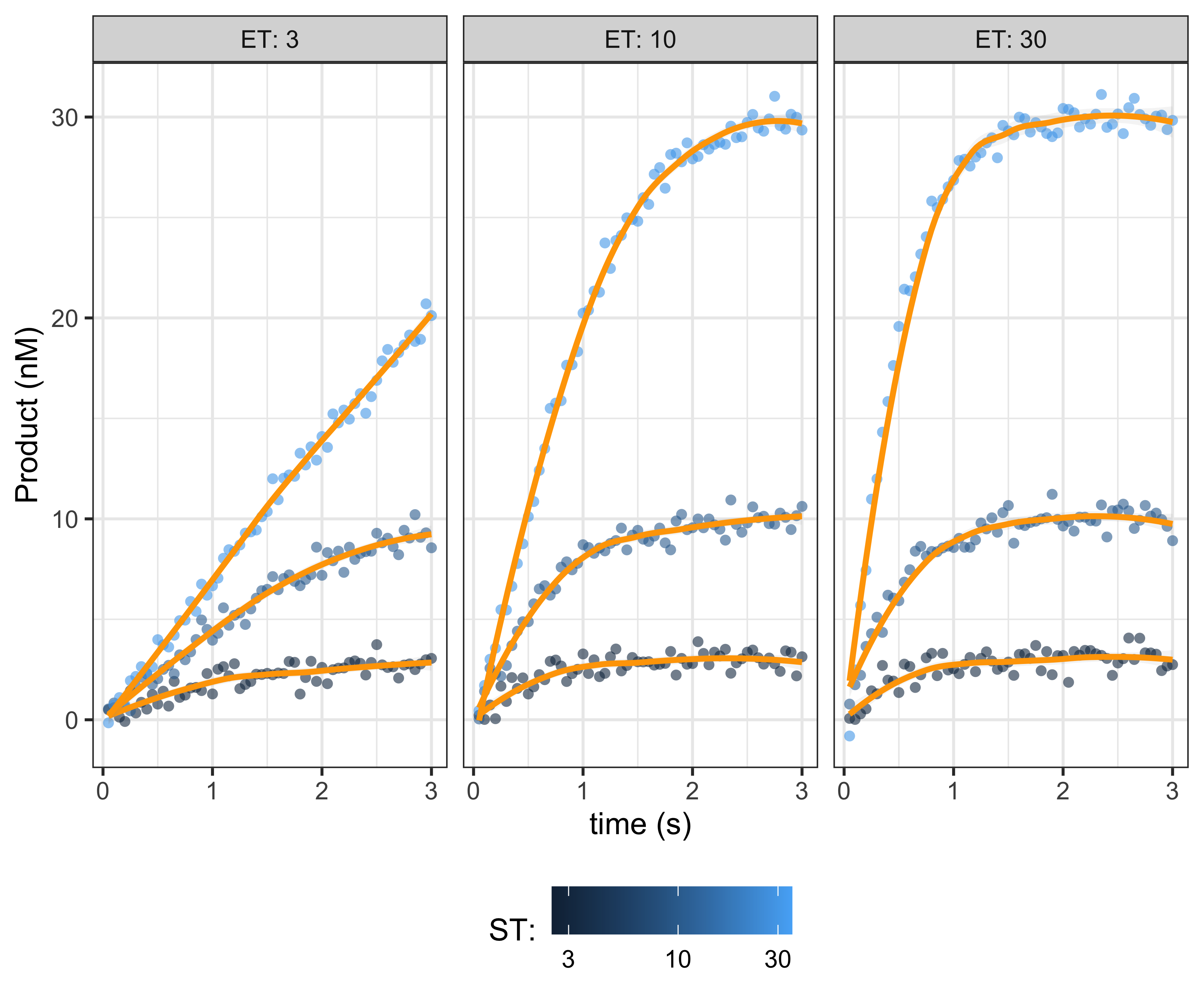

plot of chunk data-multiple-plot

stanvars_tQ_multiple <- brms::stanvar(scode = paste("
vector tQ_multiple(
  array[] int replica,
  data vector time,
  vector vkcat,
  vector vkM,
  data vector vET,
  data vector vST) {

  int N = size(time);
  vector[N] P;
  int begin = 1;
  int current_replica = replica[1];
  for (i in 1:N){
    if(current_replica != replica[i]){
      P[begin:i-1] = tQ_single(
        time[begin:i-1],
        vkcat,
        vkM,
        vET[begin:i-1],
        vST[begin:i-1]);
      begin = i;
      current_replica = replica[i];
    }
  }
  P[begin:N] = tQ_single(time[begin:N], vkcat, vkM, vET[begin:N], vST[begin:N]);
  return(P);
}", sep = "\n"),
block = "functions")

model_multiple <- do.call(what = brms::brm, args = c(list(
  formula = brms::brmsformula(
    P ~ tQ_multiple(observation_index, time, kcat, kM, ET, ST),
    kcat + kM ~ 1,
    nl = TRUE,
    loop=FALSE),
  data = data_multiple,
  prior = c(
    brms::prior(prior = gamma(4, 1), lb = 0, nlpar = "kcat"),
    brms::prior(prior = gamma(4, 1), lb = 0, nlpar = "kM")),
  init = function() list(kcat = 4, kM = 4),
  stanvars = c(
    stanvars_tQ_ode,
    stanvars_tQ_single,
    stanvars_tQ_multiple)),
  brms_params))

## Warning in '/var/folders/w2/kpys2s194q381xp3_knz9bgc0000gs/T/RtmpFnbbA1/model-141033d27a17.stan', line 34, column 2: Declaration
##     of arrays by placing brackets after a variable name is deprecated and
##     will be removed in Stan 2.33.0. Instead use the array keyword before the
##     type. This can be changed automatically using the auto-format flag to
##     stanc

## error: PCH file uses an older PCH format that is no longer supported

## Warning: CmdStan's precompiled header (PCH) files may need to be rebuilt.
## If your model failed to compile please run rebuild_cmdstan().
## If the issue persists please open a bug report.

## 1 error generated.

## make[1]: *** [/var/folders/w2/kpys2s194q381xp3_knz9bgc0000gs/T/RtmpFnbbA1/model-141033d27a17] Error 1

## Error: An error occured during compilation! See the message above for more information.

model_multiple

## Error in eval(expr, envir, enclos): object 'model_multiple' not found

## Error in eval(expr, envir, enclos): object 'model_multiple' not found

## Error in eval(expr, envir, enclos): object 'model_multiple_prior' not found

## Error in eval(expr, envir, enclos): object 'model_multiple' not found

## Error in eval(expr, envir, enclos): object 'draws_multiple_prior' not found

## Error in eval(expr, envir, enclos): object 'draws_multiple_posterior' not found

## Error in eval(expr, envir, enclos): object 'draws_multiple_prior_pairs' not found

Next we will sample enzyme progress curves from the posterior

## Error in eval(expr, envir, enclos): object 'draws_multiple_posterior' not found

## Error in eval(expr, envir, enclos): object 'sample_multiple' not found