Apply: MuSyC Model -- KCNQ Conductance
apply_MuSyC_KCNQ.RmdRe-analysis Figure 1 of (Li, et al., 2021) Molecular Basis for Ligand Activation of the Human KCNQ2 Channel
KCNQ2 is a voltage gated potassium channel important for re-establishing neuronal homeostasis following an action potential. Dis-regulation of channels in the KCNQ family can cause epilepsy, tinnitus, and depression. While there has been sustained interest in developing small-molecule based therapeutics targeting KCNQ2, the only FDA approved drug that targets KCNQ2, retigabine, was given a black-box warning due to unwanted side-effects, even though it was effective at treating epilepsy. Excitingly there has been recent progress in using Cryo-EM to structurally characterize ion channels including KCNQ2, which promise to support structure-based drug design.
Recently, (Li et al. 2021) used Cryo-EM to characterize the structure of KCNQ2 in complex with retigabine, which interacts in the membrane on the outside of the pore, and ztz240, which interacts with the voltage sensor domain. To relate the structure and function, (Li et al. 2021) measured conductance as a function of voltage (G-V curves) in the presence of varying doses of retigabine and ztz240 using whole cell patch-clamp electrophysiology in Chinese hamster ovary (CHO)-K1 cells overexpressing KCNQ2. Both compounds are thought to be agonists, that is with increasing concentration of drug, less negative voltages are required to open the channel.
In this case study, the aim is to re-analyze the effects of retigabine and ztz240 using the data collected in (Li et al. 2021) and presented in panels B and D of figure 1. A key idea is to recognize that voltage and drug treatment can be thought of independent perturbations and the drug effect can be framed as characterizing the interaction between these perturbations.
To begin, we will load and plot the data,
## # A tibble: 1,856 × 6
##    treatment dose_uM is_control voltage replica   conductance
##    <chr>       <dbl> <lgl>        <dbl> <chr>           <dbl>
##  1 ztz240         10 TRUE           -90 replica_1      0.0403
##  2 ztz240         10 TRUE           -90 replica_2      0.0632
##  3 ztz240         10 TRUE           -90 replica_3      0.0200
##  4 ztz240         10 TRUE           -90 replica_4      0.0404
##  5 ztz240         10 TRUE           -90 replica_5      0.0175
##  6 ztz240         10 TRUE           -80 replica_1      0.0469
##  7 ztz240         10 TRUE           -80 replica_2      0.0682
##  8 ztz240         10 TRUE           -80 replica_3      0.0345
##  9 ztz240         10 TRUE           -80 replica_4      0.0574
## 10 ztz240         10 TRUE           -80 replica_5      0.0339
## # ℹ 1,846 more rows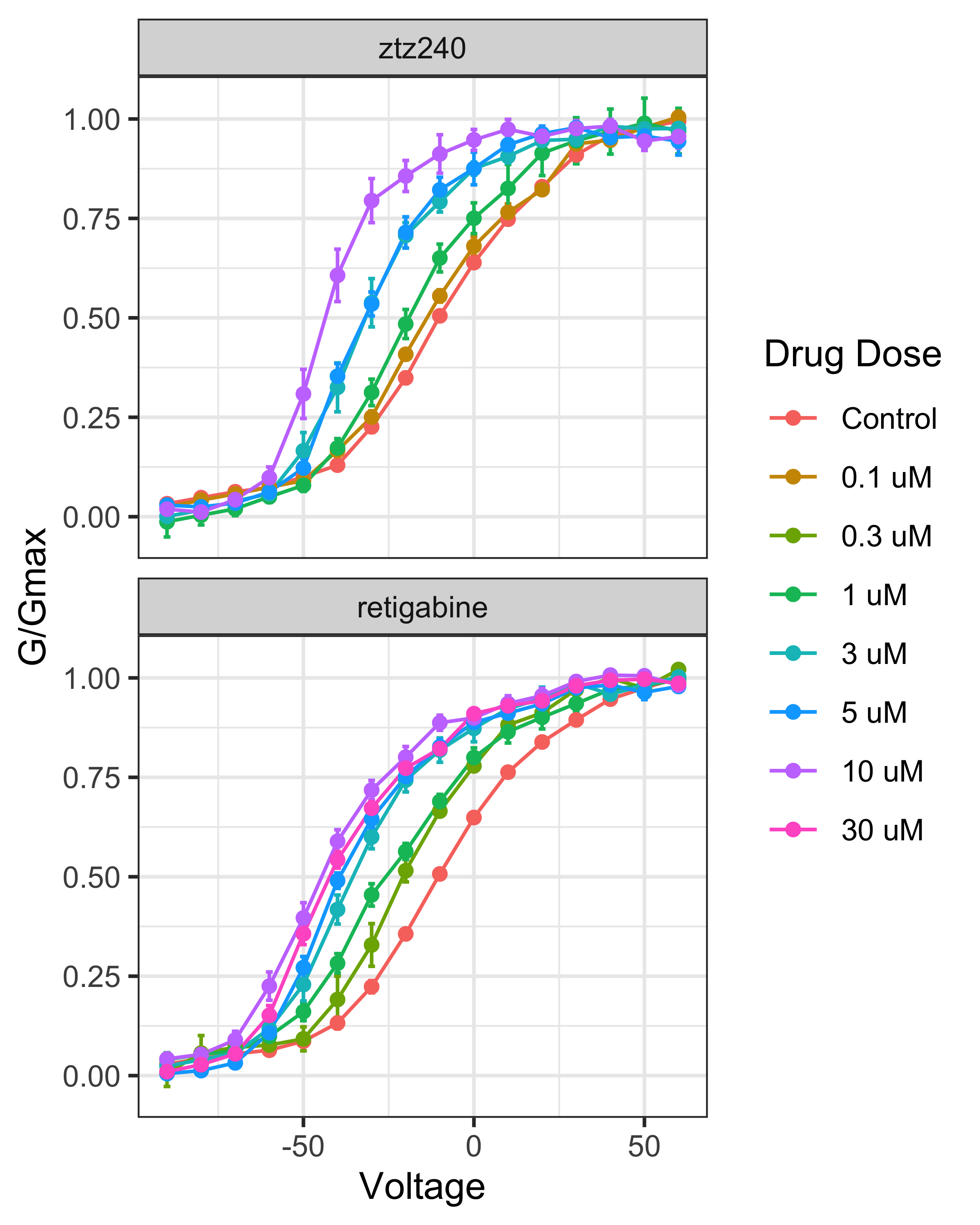
Reproduction of Figure 1b and 1d from (Li, et al., 2021)
Then, for each treatment and dose, we will fit a sigmoid curve, which has an comparable functional form to the what they call the Boltzmann equation for G/Gmax as a function of voltage. To make the fitting more stable, we will transform the treatment and response scales.
model_conductance <- BayesPharma::sigmoid_model(
  data = model_data,
  formula = BayesPharma::sigmoid_agonist_formula(
    treatment_variable = "voltage",
    treatment_units = "mV",
    response_variable = "conductance",
    response_units = "% Gmax",
    predictors = 0 + treatment:doselabel),
  prior = BayesPharma::sigmoid_agonist_prior(
    ec50 = brms::prior(normal(-0.2, 1), nlpar = "ec50"),
    hill = brms::prior(normal(3, 2), nlpar = "hill", lb = 0)),
  init = BayesPharma::sigmoid_agonist_init(
    ec50 = \() stats::runif(1, min = -7, max = -5),
    hill = \() stats::runif(1, min = 0.8, max = 1.2),
    bottom = \() stats::runif(1, min = -.1, max = 0.1),
    top = \() stats::runif(1, min = 0.8, max = 1.2)),
  cores = 4)
## Family: gaussian
## Links: mu = identity; sigma = identity
## Formula: conductance ~ sigmoid(ec50, hill, top, bottom, voltage)
## ec50 ~ 0 + treatment:doselabel
## hill ~ 0 + treatment:doselabel
## top ~ 0 + treatment:doselabel
## bottom ~ 0 + treatment:doselabel
## Data: data (Number of observations: 928)
## Draws: 4 chains, each with iter = 8000; warmup = 4000; thin = 1;
## total post-warmup draws = 16000
##
## Regression Coefficients:
## Estimate Est.Error l-95% CI u-95% CI Rhat Bulk_ESS Tail_ESS
## ec50_treatmentretigabine:doselabel0.1uM -0.21 1.01 -2.17 1.77 1.00 33343 11112
## ec50_treatmentztz240:doselabel0.1uM -0.12 0.01 -0.14 -0.09 1.00 25696 11717
## ec50_treatmentretigabine:doselabel0.3uM -0.19 0.01 -0.21 -0.17 1.00 24607 12472
## ec50_treatmentztz240:doselabel0.3uM -0.19 1.01 -2.19 1.78 1.00 35773 12326
## ec50_treatmentretigabine:doselabel1uM -0.25 0.01 -0.28 -0.22 1.00 24422 12350
## ec50_treatmentztz240:doselabel1uM -0.19 0.01 -0.22 -0.17 1.00 25285 11820
## ec50_treatmentretigabine:doselabel10uM -0.45 0.01 -0.48 -0.43 1.00 18212 11507
## ec50_treatmentztz240:doselabel10uM -0.44 0.01 -0.45 -0.42 1.00 24213 13695
## ec50_treatmentretigabine:doselabel3uM -0.36 0.01 -0.38 -0.33 1.00 21349 12088
## ec50_treatmentztz240:doselabel3uM -0.32 0.01 -0.34 -0.30 1.00 22730 12264
## ec50_treatmentretigabine:doselabel30uM -0.43 0.01 -0.46 -0.40 1.00 20758 12262
## ec50_treatmentztz240:doselabel30uM -0.20 0.99 -2.13 1.74 1.00 30655 11778
## ec50_treatmentretigabine:doselabel5uM -0.40 0.01 -0.42 -0.37 1.00 21250 11732
## ec50_treatmentztz240:doselabel5uM -0.32 0.01 -0.34 -0.30 1.00 24220 11921
## hill_treatmentretigabine:doselabel0.1uM 3.30 1.73 0.32 6.93 1.00 10612 6310
## hill_treatmentztz240:doselabel0.1uM 2.48 0.21 2.09 2.91 1.00 16355 10542
## hill_treatmentretigabine:doselabel0.3uM 3.02 0.24 2.57 3.52 1.00 16712 10445
## hill_treatmentztz240:doselabel0.3uM 3.29 1.75 0.35 6.97 1.00 11124 6646
## hill_treatmentretigabine:doselabel1uM 2.56 0.21 2.17 2.99 1.00 17215 11545
## hill_treatmentztz240:doselabel1uM 2.85 0.21 2.45 3.28 1.00 17049 11790
## hill_treatmentretigabine:doselabel10uM 2.89 0.24 2.44 3.38 1.00 15287 11263
## hill_treatmentztz240:doselabel10uM 4.99 0.44 4.20 5.92 1.00 20995 11482
## hill_treatmentretigabine:doselabel3uM 3.12 0.26 2.64 3.66 1.00 15946 11666
## hill_treatmentztz240:doselabel3uM 3.39 0.27 2.89 3.95 1.00 19724 11620
## hill_treatmentretigabine:doselabel30uM 2.78 0.22 2.37 3.21 1.00 16260 11822
## hill_treatmentztz240:doselabel30uM 3.29 1.75 0.33 6.96 1.00 10772 5933
## hill_treatmentretigabine:doselabel5uM 3.12 0.26 2.64 3.65 1.00 17214 12253
## hill_treatmentztz240:doselabel5uM 3.88 0.30 3.32 4.49 1.00 19667 11227
## top_treatmentretigabine:doselabel0.1uM 1.00 0.50 0.02 1.97 1.00 31176 10869
## top_treatmentztz240:doselabel0.1uM 0.99 0.02 0.95 1.04 1.00 17317 10739
## top_treatmentretigabine:doselabel0.3uM 0.97 0.02 0.94 1.00 1.00 18624 12117
## top_treatmentztz240:doselabel0.3uM 1.00 0.50 0.02 1.97 1.00 33883 10934
## top_treatmentretigabine:doselabel1uM 0.98 0.02 0.95 1.01 1.00 19757 10837
## top_treatmentztz240:doselabel1uM 0.93 0.01 0.90 0.96 1.00 19950 11175
## top_treatmentretigabine:doselabel10uM 0.96 0.01 0.94 0.99 1.00 21851 12955
## top_treatmentztz240:doselabel10uM 0.93 0.01 0.91 0.95 1.00 26531 12716
## top_treatmentretigabine:doselabel3uM 0.95 0.01 0.93 0.98 1.00 20730 12727
## top_treatmentztz240:doselabel3uM 0.96 0.01 0.94 0.99 1.00 23283 13128
## top_treatmentretigabine:doselabel30uM 0.96 0.01 0.94 0.99 1.00 23142 13022
## top_treatmentztz240:doselabel30uM 1.00 0.50 0.01 1.97 1.00 32862 10511
## top_treatmentretigabine:doselabel5uM 0.96 0.01 0.94 0.99 1.00 21482 11853
## top_treatmentztz240:doselabel5uM 0.95 0.01 0.93 0.98 1.00 22608 11211
## bottom_treatmentretigabine:doselabel0.1uM -0.00 0.50 -0.99 1.00 1.00 35456 11052
## bottom_treatmentztz240:doselabel0.1uM 0.01 0.02 -0.03 0.04 1.00 19646 11649
## bottom_treatmentretigabine:doselabel0.3uM 0.02 0.02 -0.02 0.05 1.00 18600 11567
## bottom_treatmentztz240:doselabel0.3uM -0.00 0.50 -0.98 0.97 1.00 34350 11024
## bottom_treatmentretigabine:doselabel1uM 0.00 0.02 -0.04 0.04 1.00 18432 11647
## bottom_treatmentztz240:doselabel1uM -0.02 0.02 -0.06 0.01 1.00 18270 10577
## bottom_treatmentretigabine:doselabel10uM -0.04 0.03 -0.10 0.02 1.00 14829 10783
## bottom_treatmentztz240:doselabel10uM -0.00 0.02 -0.04 0.03 1.00 20424 12641
## bottom_treatmentretigabine:doselabel3uM -0.01 0.02 -0.06 0.03 1.00 16697 11849
## bottom_treatmentztz240:doselabel3uM -0.02 0.02 -0.06 0.02 1.00 18232 11040
## bottom_treatmentretigabine:doselabel30uM -0.07 0.03 -0.13 -0.02 1.00 16542 11534
## bottom_treatmentztz240:doselabel30uM 0.00 0.50 -0.98 0.99 1.00 29796 10867
## bottom_treatmentretigabine:doselabel5uM -0.05 0.03 -0.10 -0.00 1.00 16662 11473
## bottom_treatmentztz240:doselabel5uM 0.00 0.02 -0.03 0.04 1.00 20056 11905
##
## Further Distributional Parameters:
## Estimate Est.Error l-95% CI u-95% CI Rhat Bulk_ESS Tail_ESS
## sigma 0.06 0.00 0.06 0.06 1.00 26451 11053
##
## Draws were sampled using sampling(NUTS). For each parameter, Bulk_ESS
## and Tail_ESS are effective sample size measures, and Rhat is the potential
## scale reduction factor on split chains (at convergence, Rhat = 1).
model_conductance |>
  BayesPharma::plot_prior_posterior_densities(refresh = 0)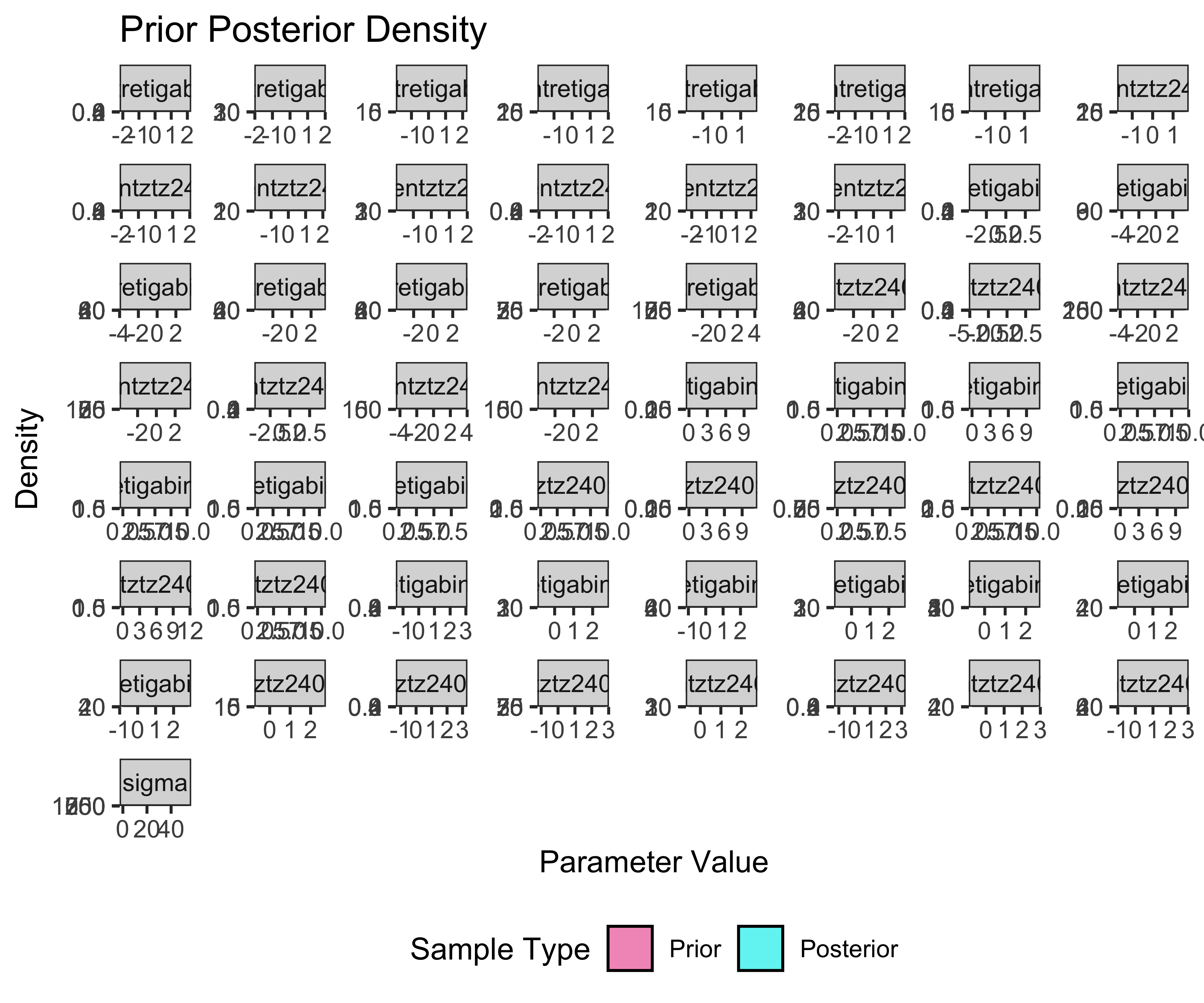
plot of chunk model-conductance-prior-posterior
model_conductance |>
  BayesPharma::plot_posterior_draws()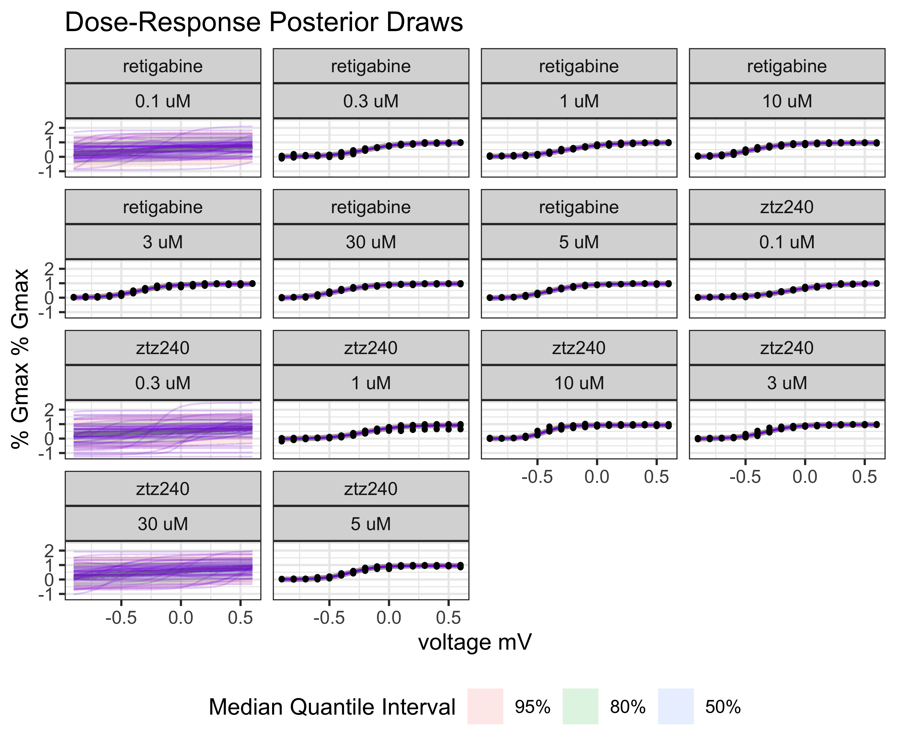
plot of chunk model-conductance-predictive
Fit MuSyC Model
Join the conductance model with the dose information to model how the voltage dependence depends on the drug dose
## # A tibble: 44 × 15
##    variable_type variable predictors_label                     mean median      sd     mad     q5     q95  rhat ess_bulk ess_tail treatment  logdose doselabel
##    <chr>         <chr>    <chr>                               <dbl>  <dbl>   <dbl>   <dbl>  <dbl>   <dbl> <dbl>    <dbl>    <dbl> <chr>        <dbl> <fct>
##  1 b             ec50     treatmentztz240:doselabel0.1uM     -0.116 -0.116 0.0147  0.0146  -0.140 -0.0916  1.00   25696.   11717. ztz240       -7    0.1 uM
##  2 b             ec50     treatmentretigabine:doselabel0.3uM -0.189 -0.189 0.0120  0.0119  -0.209 -0.170   1.00   24607.   12472. retigabine   -6.52 0.3 uM
##  3 b             ec50     treatmentretigabine:doselabel1uM   -0.247 -0.247 0.0143  0.0142  -0.271 -0.224   1.00   24422.   12350. retigabine   -6    1 uM
##  4 b             ec50     treatmentztz240:doselabel1uM       -0.194 -0.194 0.0119  0.0119  -0.214 -0.175   1.00   25285.   11820. ztz240       -6    1 uM
##  5 b             ec50     treatmentretigabine:doselabel10uM  -0.451 -0.451 0.0138  0.0137  -0.475 -0.429   1.00   18212.   11507. retigabine   -5    10 uM
##  6 b             ec50     treatmentztz240:doselabel10uM      -0.438 -0.438 0.00812 0.00803 -0.451 -0.425   1.00   24213.   13695. ztz240       -5    10 uM
##  7 b             ec50     treatmentretigabine:doselabel3uM   -0.356 -0.356 0.0123  0.0123  -0.376 -0.336   1.00   21349.   12088. retigabine   -5.52 3 uM
##  8 b             ec50     treatmentztz240:doselabel3uM       -0.322 -0.322 0.0108  0.0107  -0.340 -0.304   1.00   22730.   12264. ztz240       -5.52 3 uM
##  9 b             ec50     treatmentretigabine:doselabel30uM  -0.430 -0.430 0.0135  0.0134  -0.453 -0.408   1.00   20758.   12262. retigabine   -4.52 30 uM
## 10 b             ec50     treatmentretigabine:doselabel5uM   -0.398 -0.398 0.0122  0.0122  -0.419 -0.378   1.00   21250.   11732. retigabine   -5.30 5 uM
## # ℹ 34 more rows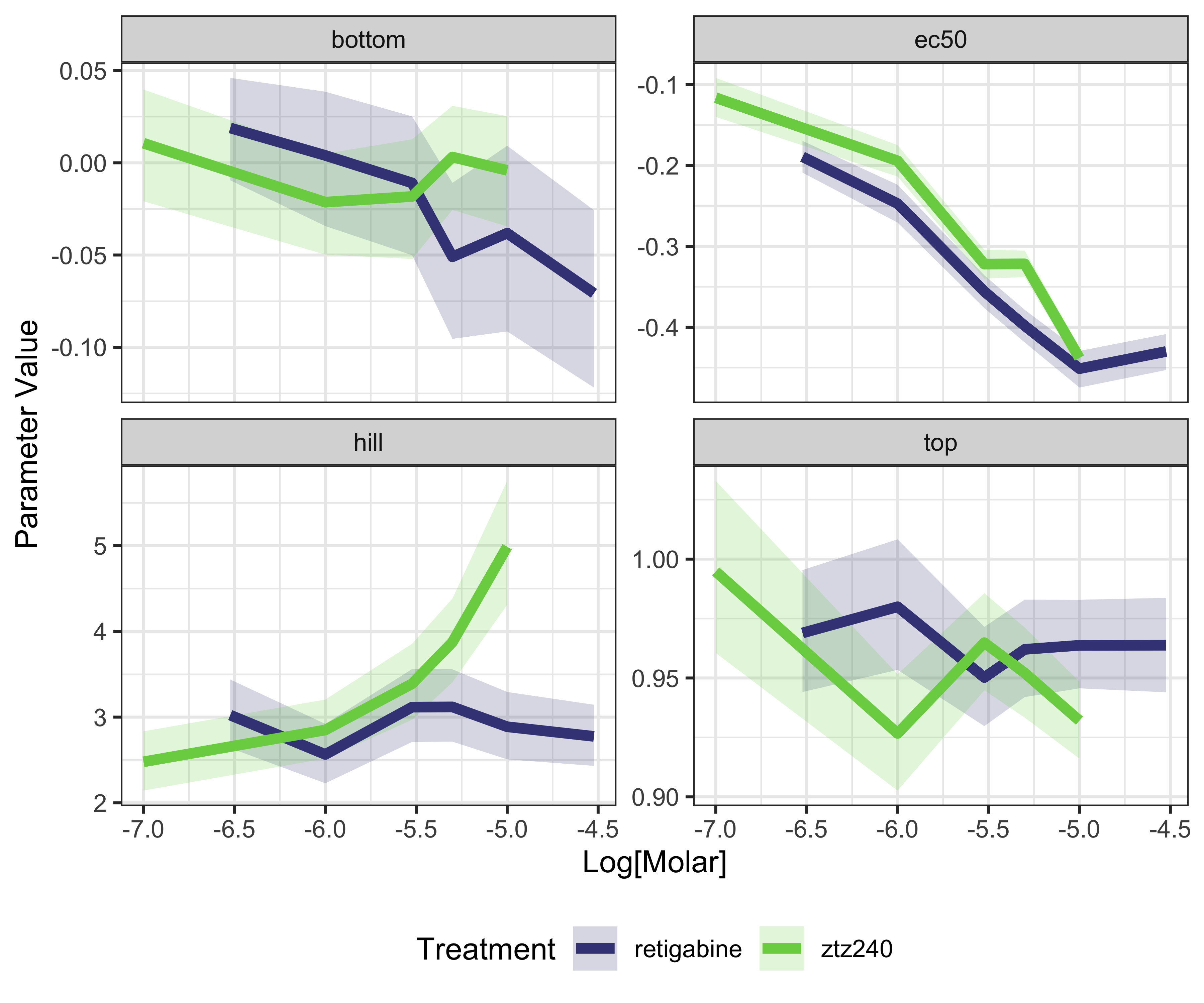
plot of chunk plot-voltage-by-dose
##  Family: gaussian
##   Links: mu = identity; sigma = identity
## Formula: conductance ~ sigmoid(sigmoid(Eec50, Ehill, Etop, Ebottom, logdose), sigmoid(Hec50, Hhill, Htop, Hbottom, logdose), vtop, vbottom, voltage)
##          vtop ~ 1
##          vbottom ~ 1
##          Eec50 ~ 0 + treatment
##          Ehill ~ 0 + treatment
##          Etop ~ 0 + treatment
##          Ebottom ~ 0 + treatment
##          Hec50 ~ 0 + treatment
##          Hhill ~ 0 + treatment
##          Htop ~ 0 + treatment
##          Hbottom ~ 0 + treatment
##    Data: model_data (Number of observations: 928)
##   Draws: 4 chains, each with iter = 2000; warmup = 1000; thin = 1;
##          total post-warmup draws = 4000
##
## Regression Coefficients:
##                             Estimate Est.Error l-95% CI u-95% CI Rhat Bulk_ESS Tail_ESS
## vtop_Intercept                  0.95      0.00     0.95     0.96 1.00     4877     3132
## vbottom_Intercept              -0.00      0.01    -0.01     0.01 1.00     4746     2892
## Eec50_treatmentretigabine      -5.77      0.07    -5.92    -5.65 1.00     2291     1855
## Eec50_treatmentztz240          -5.46      0.06    -5.56    -5.34 1.00     2283     1906
## Ehill_treatmentretigabine      -1.62      0.27    -2.17    -1.12 1.00     2220     1885
## Ehill_treatmentztz240          -1.45      0.17    -1.82    -1.15 1.00     2259     2164
## Etop_treatmentretigabine       -0.19      0.02    -0.22    -0.15 1.00     2017     1546
## Etop_treatmentztz240           -0.13      0.01    -0.15    -0.12 1.00     3284     2429
## Ebottom_treatmentretigabine    -0.43      0.01    -0.44    -0.41 1.00     3745     2603
## Ebottom_treatmentztz240        -0.48      0.02    -0.54    -0.44 1.00     2031     1760
## Hec50_treatmentretigabine      -3.88      1.74    -7.73    -0.37 1.00     1157     1770
## Hec50_treatmentztz240          -5.14      0.21    -5.52    -4.70 1.00     2603     2589
## Hhill_treatmentretigabine       1.28      0.74     0.23     3.00 1.00     2706     1922
## Hhill_treatmentztz240           1.78      0.49     1.02     2.93 1.00     3078     2899
## Htop_treatmentretigabine        4.49      1.63     2.27     8.33 1.00     2205     2201
## Htop_treatmentztz240            5.84      1.15     4.28     8.57 1.00     2641     2381
## Hbottom_treatmentretigabine     2.99      0.09     2.81     3.16 1.00     2134     2719
## Hbottom_treatmentztz240         2.84      0.08     2.68     2.99 1.00     4716     2988
##
## Further Distributional Parameters:
##       Estimate Est.Error l-95% CI u-95% CI Rhat Bulk_ESS Tail_ESS
## sigma     0.06      0.00     0.06     0.06 1.00     4626     2683
##
## Draws were sampled using sampling(NUTS). For each parameter, Bulk_ESS
## and Tail_ESS are effective sample size measures, and Rhat is the potential
## scale reduction factor on split chains (at convergence, Rhat = 1).
## elpd_diff se_diff
## model_bilevel 0.0 0.0
## model_MuSyC -125.4 17.2## Re-fitting the models with only 0.01 fraction of the data## Warning: There were 2 divergent transitions after warmup. See
## https://mc-stan.org/misc/warnings.html#divergent-transitions-after-warmup
## to find out why this is a problem and how to eliminate them.## Warning: Examine the pairs() plot to diagnose sampling problems## Re-fitting the models with only 0.02 fraction of the data
## Re-fitting the models with only 0.03 fraction of the data## Warning: Some Pareto k diagnostic values are too high. See help('pareto-k-diagnostic') for details.## Warning: Found 1 observations with a pareto_k > 0.7 in model 'stats::update(model_bilevel, newdata = model_data_subset, cores = 4, control = list(adapt_delta = 0.99, max_treedepth = 12), silent = TRUE)'. We recommend to set 'reloo = TRUE' in order to calculate the ELPD without the assumption that
## these observations are negligible. This will refit the model 1 times to compute the ELPDs for the problematic observations directly.## Re-fitting the models with only 0.04 fraction of the data## Warning: Some Pareto k diagnostic values are too high. See help('pareto-k-diagnostic') for details.
## Warning: Found 1 observations with a pareto_k > 0.7 in model 'stats::update(model_bilevel, newdata = model_data_subset, cores = 4, control = list(adapt_delta = 0.99, max_treedepth = 12), silent = TRUE)'. We recommend to set 'reloo = TRUE' in order to calculate the ELPD without the assumption that these observations are negligible. This will refit the model 1 times to compute the ELPDs for the problematic observations directly.## Re-fitting the models with only 0.05 fraction of the data## Warning: Bulk Effective Samples Size (ESS) is too low, indicating posterior means and medians may be unreliable.
## Running the chains for more iterations may help. See
## https://mc-stan.org/misc/warnings.html#bulk-ess## Warning: Tail Effective Samples Size (ESS) is too low, indicating posterior variances and tail quantiles may be unreliable.
## Running the chains for more iterations may help. See
## https://mc-stan.org/misc/warnings.html#tail-ess## Re-fitting the models with only 0.06 fraction of the data
## Re-fitting the models with only 0.07 fraction of the data
## Re-fitting the models with only 0.08 fraction of the data## Warning: The largest R-hat is NA, indicating chains have not mixed.
## Running the chains for more iterations may help. See
## https://mc-stan.org/misc/warnings.html#r-hat## Warning: Bulk Effective Samples Size (ESS) is too low, indicating posterior means and medians may be unreliable.
## Running the chains for more iterations may help. See
## https://mc-stan.org/misc/warnings.html#bulk-ess## Warning: Tail Effective Samples Size (ESS) is too low, indicating posterior variances and tail quantiles may be unreliable.
## Running the chains for more iterations may help. See
## https://mc-stan.org/misc/warnings.html#tail-ess## Warning: Some Pareto k diagnostic values are too high. See help('pareto-k-diagnostic') for details.## Warning: Found 1 observations with a pareto_k > 0.7 in model 'stats::update(model_MuSyC, newdata = dplyr::mutate(model_data_subset, logd1scale = mean(voltage), logd2scale = mean(logdose)), control = list(adapt_delta = 0.99, max_treedepth = 12), cores = 4, silent = TRUE)'. We recommend to set 'reloo
## = TRUE' in order to calculate the ELPD without the assumption that these observations are negligible. This will refit the model 1 times to compute the ELPDs for the problematic observations directly.## Re-fitting the models with only 0.09 fraction of the data## Warning: The largest R-hat is NA, indicating chains have not mixed.
## Running the chains for more iterations may help. See
## https://mc-stan.org/misc/warnings.html#r-hat## Warning: Bulk Effective Samples Size (ESS) is too low, indicating posterior means and medians may be unreliable.
## Running the chains for more iterations may help. See
## https://mc-stan.org/misc/warnings.html#bulk-ess## Warning: Tail Effective Samples Size (ESS) is too low, indicating posterior variances and tail quantiles may be unreliable.
## Running the chains for more iterations may help. See
## https://mc-stan.org/misc/warnings.html#tail-ess## Warning: There were 1 divergent transitions after warmup. See
## https://mc-stan.org/misc/warnings.html#divergent-transitions-after-warmup
## to find out why this is a problem and how to eliminate them.## Warning: Examine the pairs() plot to diagnose sampling problems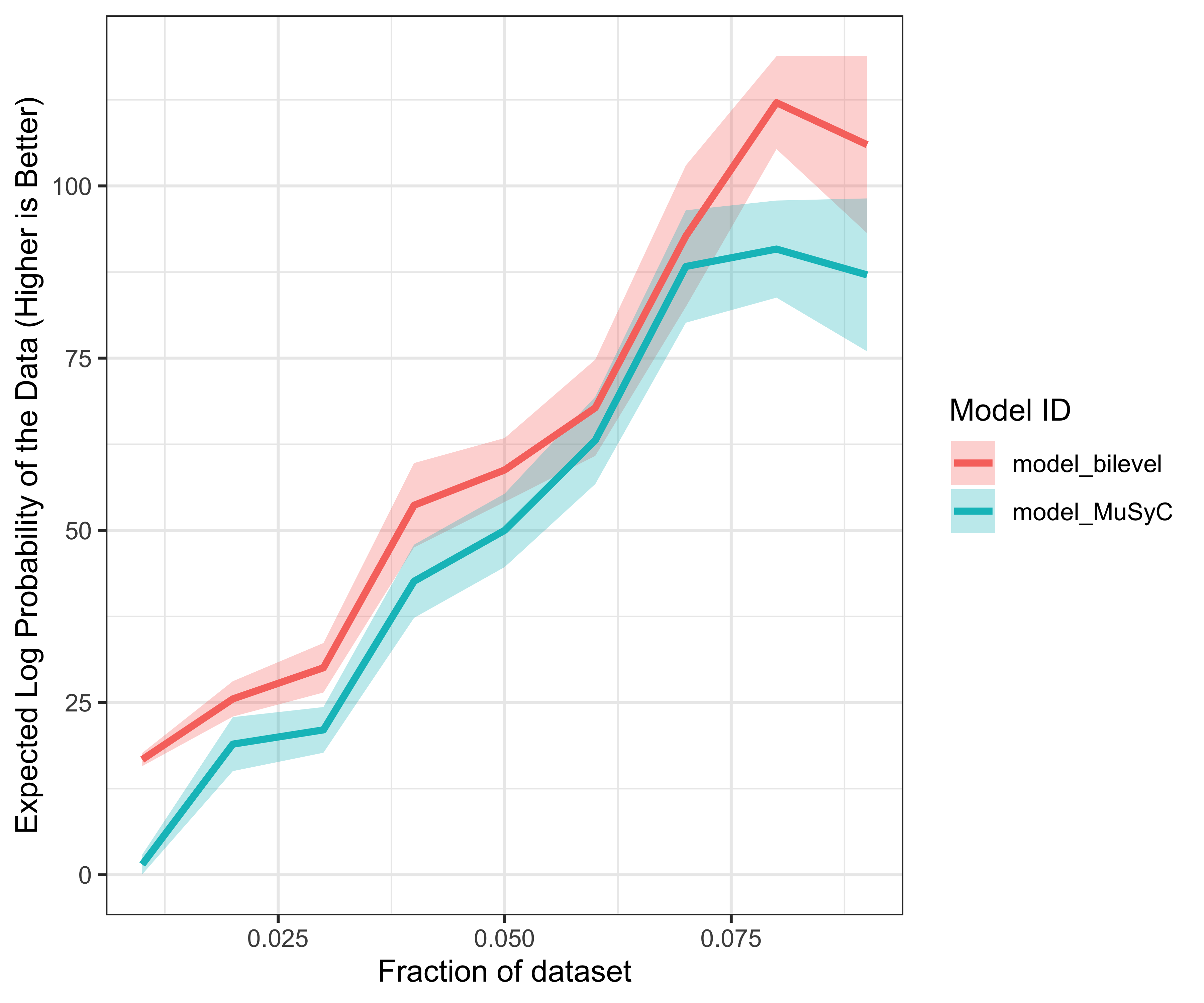
plot of chunk model-data-subset